Note
Click here to download the full example code
Rampp event detection#
This example illustrates how the gait event detection by the RamppEventDetection or
FilteredRamppEventDetection can be used to detect gait events within a list of strides
and the corresponding IMU signal.
The used implementation is based on the work of Rampp et al. [1].
Getting some example data#
For this we take some example data that contains the regular walking movement during a 2x20m walk test of a healthy subject. The IMU signals are already rotated so that they align with the gaitmap SF coordinate system. The data contains information from two sensors - one from the right and one from the left foot. For further information regarding the coordinate system refer to the coordinate system guide.
from gaitmap.example_data import get_healthy_example_imu_data

data = get_healthy_example_imu_data()
sampling_rate_hz = 204.8
data.sort_index(axis=1).head(1)
Getting the example stride list#
For this we take the ground truth stride list provided with the example data. For new data this stride list can be
generated by running the algorithms provided in the stride_segmentation module.
from gaitmap.example_data import get_healthy_example_stride_borders

stride_list = get_healthy_example_stride_borders()

stride_list["left_sensor"].head()
Preparing the data#
The data is expected to be in the gaitmap BF to be able to use the same template for the left and the right foot. Therefore, we need to transform the our dataset into the body frame. For further information regarding the coordinate system refer to the coordinate system guide.
from gaitmap.utils.coordinate_conversion import convert_to_fbf

# We use the `..._like` parameters to identify the data of the left and the right foot based on the name of the sensor.
bf_data = convert_to_fbf(data, left_like="left_", right_like="right_")
Applying the event detection#
First we need to initialize the Rampp event detection. In most cases it is sufficient to keep all parameters at default. The default search window for the initial contact is set to 80 ms before and 50 ms after the local minimum in the gyr_ml signal. The default window size for the minimal velocity is set to 100 ms with 50 % overlap. Those default values are different from the original paper, but have proven to be useful in daily life usage.
from gaitmap.event_detection import RamppEventDetection

ed = RamppEventDetection()
# apply the event detection to the data
ed = ed.detect(data=bf_data, stride_list=stride_list, sampling_rate_hz=sampling_rate_hz)
Inspecting the results#
The main output is the min_vel_event_list_, which contains the samples of initial contact (ic), terminal contact
(tc), and minimal velocity (min_vel) formatted in a way that can be directly used for a stride-level trajectory
reconstruction.
The start sample of each stride corresponds to the min_vel sample of that stride and the end sample corresponds to the
min_vel sample of the subsequent stride.
Furthermore, the min_vel_event_list_ list provides the pre_ic which is the ic event of the previous stride in the
stride list.
As we passed a dataset with two sensors, the output will be a dictionary.
min_vel_events_left = ed.min_vel_event_list_["left_sensor"]
print(f"Gait events for {len(min_vel_events_left)} min_vel strides were detected.")
min_vel_events_left.head()
Gait events for 26 min_vel strides were detected.
As a secondary output we get the segmented_event_list_, which holds the same event information than the
min_vel_event_list_, but the start and the end of each stride are unchanged compared to the input.
This also means that no strides are removed due to the conversion step explained below.
segmented_events_left = ed.segmented_event_list_["left_sensor"]
print(f"Gait events for {len(segmented_events_left)} segmented strides were detected.")
segmented_events_left.head()
Gait events for 28 segmented strides were detected.
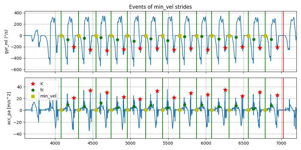
To get a better understanding of the results, we can plot the data and the gait events.
The top row shows the gyr_ml axis, the lower row the acc_pa axis along with the gait events with indicators as
described in the plot legend.
The vertical lines show the start and end of the strides that are overlapping with the min_vel samples.
Only the second sequence of strides of the left foot are shown.
import matplotlib.pyplot as plt

fig, (ax1, ax2) = plt.subplots(2, sharex=True, figsize=(10, 5))
ax1.plot(bf_data.reset_index(drop=True)["left_sensor"][["gyr_ml"]])
ax2.plot(bf_data.reset_index(drop=True)["left_sensor"][["acc_pa"]])

ic_idx = ed.min_vel_event_list_["left_sensor"]["ic"].to_numpy().astype(int)
tc_idx = ed.min_vel_event_list_["left_sensor"]["tc"].to_numpy().astype(int)
min_vel_idx = ed.min_vel_event_list_["left_sensor"]["min_vel"].to_numpy().astype(int)

for ax, sensor in zip([ax1, ax2], ["gyr_ml", "acc_pa"]):
    for _i, stride in ed.min_vel_event_list_["left_sensor"].iterrows():
        ax.axvline(stride["start"], color="g")
        ax.axvline(stride["end"], color="r")

    ax.scatter(
        ic_idx,
        bf_data["left_sensor"][sensor].to_numpy()[ic_idx],
        marker="*",
        s=100,
        color="r",
        zorder=3,
        label="ic",
    )

    ax.scatter(
        tc_idx,
        bf_data["left_sensor"][sensor].to_numpy()[tc_idx],
        marker="p",
        s=50,
        color="g",
        zorder=3,
        label="tc",
    )

    ax.scatter(
        min_vel_idx,
        bf_data["left_sensor"][sensor].to_numpy()[min_vel_idx],
        marker="s",
        s=50,
        color="y",
        zorder=3,
        label="min_vel",
    )

    ax.grid(True)

ax1.set_title("Events of min_vel strides")
ax1.set_ylabel("gyr_ml (°/s)")
ax2.set_ylabel("acc_pa [m/s^2]")
ax1.set_xlim(3600, 7200)
# ax1.set_xlim(1150, 1850)
plt.legend(loc="best")

fig.tight_layout()
fig.show()
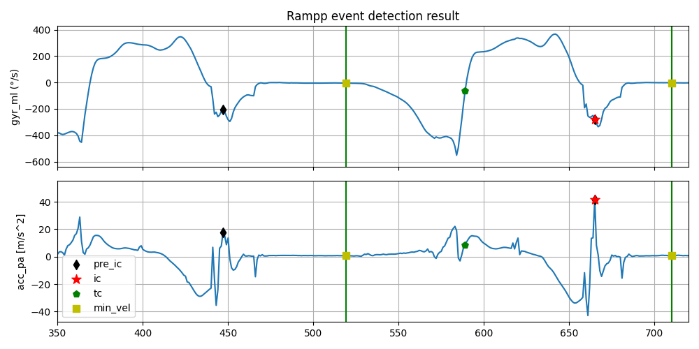
To better understand the concept of ic and pre_ic, let’s take a closer look at the data and zoom in a bit more. We can see now that every stride has a pre_ic and especially in case of the first stride of a sequence this pre_ic is not an ic for any stride. It only serves as a pre_ic for the subsequent stride.
fig, (ax1, ax2) = plt.subplots(2, sharex=True, figsize=(10, 5))
ax1.plot(bf_data.reset_index(drop=True)["left_sensor"][["gyr_ml"]])
ax2.plot(bf_data.reset_index(drop=True)["left_sensor"][["acc_pa"]])

pre_ic_idx = ed.min_vel_event_list_["left_sensor"]["pre_ic"].to_numpy().astype(int)

for ax, sensor in zip([ax1, ax2], ["gyr_ml", "acc_pa"]):
    for _i, stride in ed.min_vel_event_list_["left_sensor"].iterrows():
        ax.axvline(stride["start"], color="g")
        ax.axvline(stride["end"], color="r")

    ax.scatter(
        pre_ic_idx,
        bf_data["left_sensor"][sensor].to_numpy()[pre_ic_idx],
        marker="d",
        s=50,
        color="k",
        zorder=3,
        label="pre_ic",
    )

    ax.scatter(
        ic_idx,
        bf_data["left_sensor"][sensor].to_numpy()[ic_idx],
        marker="*",
        s=100,
        color="r",
        zorder=3,
        label="ic",
    )

    ax.scatter(
        tc_idx,
        bf_data["left_sensor"][sensor].to_numpy()[tc_idx],
        marker="p",
        s=50,
        color="g",
        zorder=3,
        label="tc",
    )

    ax.scatter(
        min_vel_idx,
        bf_data["left_sensor"][sensor].to_numpy()[min_vel_idx],
        marker="s",
        s=50,
        color="y",
        zorder=3,
        label="min_vel",
    )

    ax.grid(True)

ax1.set_title("Rampp event detection result")
ax1.set_ylabel("gyr_ml (°/s)")
ax2.set_ylabel("acc_pa [m/s^2]")
ax1.set_xlim(350, 720)
plt.legend(loc="best")

fig.tight_layout()
fig.show()
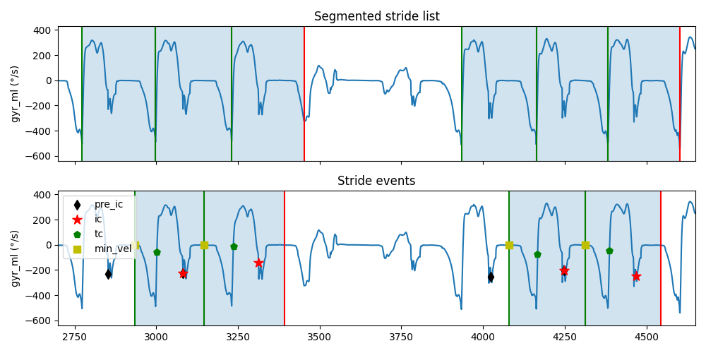
Furthermore, breaks in continuous gait sequences (with continuous subsequent strides according to the stride_list)
are detected and the first (segmented) stride of each sequence is dropped.
This is required due to the shift of stride borders between the stride_list and the min_vel_event_list_.
Thus, the dropped first segmented stride of a continuous sequence only provides a pre_ic and a min_vel sample for
the first stride in the min_vel_event_list_.
Therefore, the min_vel_event_list_ list has one stride less than the segmented_event_list_.
from gaitmap.event_detection import RamppEventDetection

ed2 = RamppEventDetection()
segmented_stride_list = stride_list["left_sensor"].iloc[[11, 12, 13, 14, 15, 16]]
ed2.detect(
    data=bf_data["left_sensor"],
    sampling_rate_hz=sampling_rate_hz,
    stride_list=segmented_stride_list,
)

fig, (ax1, ax2) = plt.subplots(2, sharex=True, figsize=(10, 5))

sensor_axis = "gyr_ml"

ax1.plot(bf_data.reset_index(drop=True)["left_sensor"][sensor_axis])
for _i, stride in segmented_stride_list.iterrows():
    ax1.axvline(stride["start"], color="g")
    ax1.axvline(stride["end"], color="r")
    ax1.axvspan(stride["start"], stride["end"], alpha=0.2)

ax2.plot(bf_data.reset_index(drop=True)["left_sensor"][sensor_axis])

ic_idx = ed2.min_vel_event_list_["ic"].to_numpy().astype(int)
tc_idx = ed2.min_vel_event_list_["tc"].to_numpy().astype(int)
min_vel_idx = ed2.min_vel_event_list_["min_vel"].to_numpy().astype(int)
pre_ic_idx = ed2.min_vel_event_list_["pre_ic"].to_numpy().astype(int)

for _i, stride in ed2.min_vel_event_list_.iterrows():
    ax2.axvline(stride["start"], color="g")
    ax2.axvline(stride["end"], color="r")
    ax2.axvspan(stride["start"], stride["end"], alpha=0.2)

ax2.scatter(
    pre_ic_idx,
    bf_data["left_sensor"][sensor_axis].to_numpy()[pre_ic_idx],
    marker="d",
    s=50,
    color="k",
    zorder=3,
    label="pre_ic",
)

ax2.scatter(
    ic_idx,
    bf_data["left_sensor"][sensor_axis].to_numpy()[ic_idx],
    marker="*",
    s=100,
    color="r",
    zorder=3,
    label="ic",
)

ax2.scatter(
    tc_idx,
    bf_data["left_sensor"][sensor_axis].to_numpy()[tc_idx],
    marker="p",
    s=50,
    color="g",
    zorder=3,
    label="tc",
)

ax2.scatter(
    min_vel_idx,
    bf_data["left_sensor"][sensor_axis].to_numpy()[min_vel_idx],
    marker="s",
    s=50,
    color="y",
    zorder=3,
    label="min_vel",
)

ax1.set_title("Segmented stride list")
ax1.set_ylabel("gyr_ml (°/s)")
ax2.set_title("Stride events")
ax2.set_ylabel("gyr_ml (°/s)")
ax1.set_xlim(2700, 4650)
fig.tight_layout()

plt.legend(loc="upper left")
fig.show()

from gaitmap.data_transform import ButterworthFilter
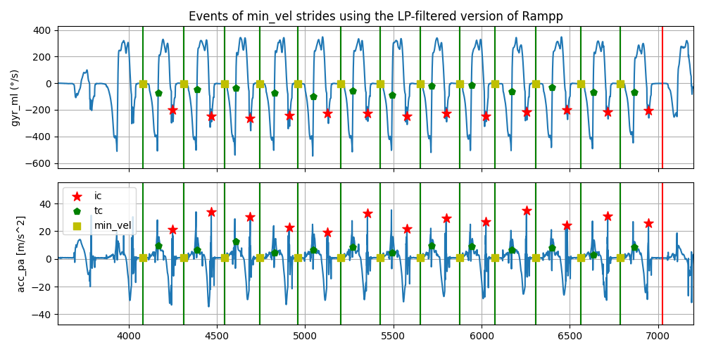
Filtered Rampp Event Detection#
For signals with high frequency noise and artifact the FilteredRamppEventDetection
can be used.
A low pass filter is implemented in this class and is applied on the gyr-ml signal for detecting IC.
The IC searches for the “valley” after the swing peak in gyr_ml.
The high frequency components near the vally might result in the false detection of IC.
For changing the filter parameters a tuple should pass to ic_lowpass_filter.
For this data you don’t see a difference.
However, when you encounter issues, testing the filtered version might be an option.
from gaitmap.event_detection import FilteredRamppEventDetection

edfilt = FilteredRamppEventDetection(ic_lowpass_filter=ButterworthFilter(10, 15))
edfilt = edfilt.detect(data=bf_data, stride_list=stride_list, sampling_rate_hz=sampling_rate_hz)
min_vel_events_left = edfilt.min_vel_event_list_["left_sensor"]
print(f"Gait events for {len(min_vel_events_left)} min_vel strides using the filtered version were detected.")
min_vel_events_left.head()
segmented_events_left = edfilt.segmented_event_list_["left_sensor"]
print(f"Gait events for {len(segmented_events_left)} segmented strides using the filtered version were detected.")
segmented_events_left.head()
fig, (ax1, ax2) = plt.subplots(2, sharex=True, figsize=(10, 5))
ax1.plot(bf_data.reset_index(drop=True)["left_sensor"][["gyr_ml"]])
ax2.plot(bf_data.reset_index(drop=True)["left_sensor"][["acc_pa"]])

ic_idx = edfilt.min_vel_event_list_["left_sensor"]["ic"].to_numpy().astype(int)
tc_idx = edfilt.min_vel_event_list_["left_sensor"]["tc"].to_numpy().astype(int)
min_vel_idx = edfilt.min_vel_event_list_["left_sensor"]["min_vel"].to_numpy().astype(int)

for ax, sensor in zip([ax1, ax2], ["gyr_ml", "acc_pa"]):
    for _i, stride in edfilt.min_vel_event_list_["left_sensor"].iterrows():
        ax.axvline(stride["start"], color="g")
        ax.axvline(stride["end"], color="r")

    ax.scatter(
        ic_idx,
        bf_data["left_sensor"][sensor].to_numpy()[ic_idx],
        marker="*",
        s=100,
        color="r",
        zorder=3,
        label="ic",
    )

    ax.scatter(
        tc_idx,
        bf_data["left_sensor"][sensor].to_numpy()[tc_idx],
        marker="p",
        s=50,
        color="g",
        zorder=3,
        label="tc",
    )

    ax.scatter(
        min_vel_idx,
        bf_data["left_sensor"][sensor].to_numpy()[min_vel_idx],
        marker="s",
        s=50,
        color="y",
        zorder=3,
        label="min_vel",
    )

    ax.grid(True)

ax1.set_title("Events of min_vel strides using the LP-filtered version of Rampp")
ax1.set_ylabel("gyr_ml (°/s)")
ax2.set_ylabel("acc_pa [m/s^2]")
ax1.set_xlim(3600, 7200)
# ax1.set_xlim(1150, 1850)
plt.legend(loc="best")

fig.tight_layout()
fig.show()
Gait events for 26 min_vel strides using the filtered version were detected.
Gait events for 28 segmented strides using the filtered version were detected.
Total running time of the script: ( 0 minutes 4.851 seconds)
Estimated memory usage: 9 MB