Mahony and Madgwick Orientation Estimation

This example compares MahonyAHRS and MadgwickAHRS on the same single-sensor recording. Both algorithms estimate orientation directly from IMU data, but they use different feedback mechanisms: Mahony applies proportional-integral feedback, while Madgwick uses a gradient-descent correction step.

Getting input data

We use a short section of the left foot IMU example data. The data is already aligned to the gaitmap sensor frame and contains accelerometer and gyroscope signals.

import matplotlib.pyplot as plt
import pandas as pd

from gaitmap.example_data import get_healthy_example_imu_data
from gaitmap.trajectory_reconstruction import MadgwickAHRS, MahonyAHRS

imu_data = get_healthy_example_imu_data()["left_sensor"].iloc[500:900]
sampling_frequency_hz = 204.8

Configuring and running both algorithms

kp controls how strongly the instantaneous accelerometer based correction is applied in Mahony. ki enables an accumulated bias correction term. Madgwick uses beta to control the correction strength.

mahony = MahonyAHRS(kp=0.8, ki=0.02)
madgwick = MadgwickAHRS(beta=0.2)

mahony = mahony.estimate(imu_data, sampling_rate_hz=sampling_frequency_hz)
madgwick = madgwick.estimate(imu_data, sampling_rate_hz=sampling_frequency_hz)

mahony_orientation = mahony.orientation_
madgwick_orientation = madgwick.orientation_
mahony_rotated_data = mahony.rotated_data_
madgwick_rotated_data = madgwick.rotated_data_

orientation_comparison = pd.concat(
    [mahony_orientation.add_prefix("mahony_"), madgwick_orientation.add_prefix("madgwick_")], axis=1
)
rotated_data_comparison = pd.concat(
    [mahony_rotated_data.add_prefix("mahony_"), madgwick_rotated_data.add_prefix("madgwick_")], axis=1
)

Inspecting the results

orientation_comparison.tail()

	mahony_q_x	mahony_q_y	mahony_q_z	mahony_q_w	madgwick_q_x	madgwick_q_y	madgwick_q_z	madgwick_q_w
sample
396	0.034201	-0.123389	0.009840	0.991720	0.093027	-0.106233	0.008683	0.989942
397	0.036344	-0.117614	0.008073	0.992361	0.094949	-0.100070	0.007148	0.990414
398	0.038364	-0.112578	0.006401	0.992881	0.096649	-0.094321	0.005678	0.990823
399	0.040413	-0.107899	0.004685	0.993329	0.098965	-0.088883	0.004106	0.991105
400	0.042394	-0.103143	0.003031	0.993758	0.100951	-0.083484	0.002615	0.991379

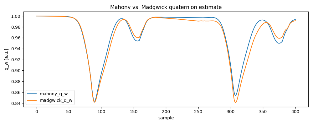
Comparing the quaternion course can help to spot how strongly both filters react to the same movement.

orientation_comparison[["mahony_q_w", "madgwick_q_w"]].plot(figsize=(10, 4))
plt.xlabel("sample")
plt.ylabel("q_w [a.u.]")
plt.title("Mahony vs. Madgwick quaternion estimate")
plt.tight_layout()
plt.show()

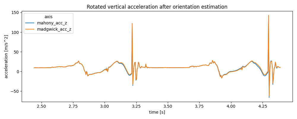
The rotated accelerometer data is often easier to interpret, because the sensor axes are aligned with the estimated global frame.

rotated_data_comparison[["mahony_acc_z", "madgwick_acc_z"]].plot(figsize=(10, 4))
plt.xlabel("time [s]")
plt.ylabel("acceleration [m/s^2]")
plt.title("Rotated vertical acceleration after orientation estimation")
plt.tight_layout()
plt.show()

Estimated memory usage: 19 MB