Stride segmentation with Regions of Interest

In long datasets it might be desirable to predefine regions of interest in which strides should be segmented. This can massively speed up the computation or focus the analysis on a specific part of the data.

Most of the time such regions of interest would be defined using some sort of gait detection algorithms (e.g. UllrichGaitSequenceDetection). In this example we will create an example output of such an algorithms and will use it to limit the search region for the BarthDtw stride segmentation algorithms. However, all other stride segmentation algorithms should this functionality as well.

Note, that for smaller datasets, the algorithms might actually be slower when using multiple regions of interest, compared to analysing the entire dataset. This is, because the method relies on a slow Python loop to process the individual regions of interest.

import matplotlib.pyplot as plt
import numpy

numpy.random.seed(0)

Getting some example data

For this we take some example data that contains the regular walking movement during a 2x20m walk test of a healthy subject. The IMU signals are already rotated so that they align with the gaitmap SF coordinate system. The data contains information from two sensors - one from the right and one from the left foot. We will further convert the data into the body frame, as this is required by the BarthDTW method to perform the stride segmentation.

from gaitmap.example_data import get_healthy_example_imu_data
from gaitmap.utils.coordinate_conversion import convert_to_fbf

data = get_healthy_example_imu_data()
sampling_rate_hz = 204.8
bf_data = convert_to_fbf(data, left_like="left_", right_like="right_")


data.sort_index(axis=1).head(1)

sensor	left_sensor						right_sensor
axis	acc_x	acc_y	acc_z	gyr_x	gyr_y	gyr_z	acc_x	acc_y	acc_z	gyr_x	gyr_y	gyr_z
0.0	0.880811	2.762208	9.40865	-0.112402	-0.032157	-0.062261	0.311553	-2.398646	9.513275	-0.323037	0.084604	-0.025288

Defining regions of interest

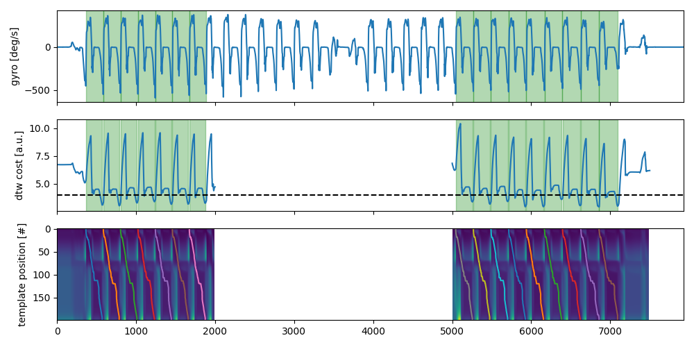
We will define two regions of interest (one at the beginning and one at the end of the dataset). We expect the algorithm to only find strides in these regions.

import pandas as pd

roi = pd.DataFrame([[0, 2000], [5000, 7500]], columns=["start", "end"])
roi.index.name = "roi_id"
roi

	start	end
roi_id
0	0	2000
1	5000	7500

Setting up the Stride Segmentation

We will use BarthDTW with the default settings.

from gaitmap.stride_segmentation import BarthDtw

dtw = BarthDtw()

Setting up the ROI wrapper

To apply our method to multiple regions of interest wie use the RoiStrideSegmentation wrapper.

from gaitmap.stride_segmentation import RoiStrideSegmentation

roi_seg = RoiStrideSegmentation(segmentation_algorithm=dtw)

Applying the segmentation

Instead of our original dtw object we now use the wrapper with the same inputs to segment.

roi_seg = roi_seg.segment(data=bf_data, sampling_rate_hz=sampling_rate_hz, regions_of_interest=roi)

Inspecting the results

The wrapper will automatically combine all stride lists from all ROIs into one. The additional “roi_id” column indicates in which ROI a stride was identified in.

stride_list_left = roi_seg.stride_list_["left_sensor"]
print(f"{len(stride_list_left)} strides were detected.")
stride_list_left

16 strides were detected.

	roi_id	start	end
s_id
0	0	364	584
1	0	584	802
2	0	802	1023
3	0	1023	1242
4	0	1242	1458
5	0	1458	1672
6	0	1672	1887
7	1	5043	5267
8	1	5267	5489
9	1	5489	5713
10	1	5713	5936
11	1	5936	6167
12	1	6167	6395
13	1	6395	6628
14	1	6628	6858
15	1	6858	7091

All other outputs of our stride segmentation method are not accumulated, as they differ from method to method. However, we can inspect the individual instances stored in the instances_per_roi_ attribute to get this information.

In the following we will plot the cost matrices that are created for ROI. We will see that we now have multiple cost matrices and cost functions per sensor. This is simply because the DTW was applied separately to the two regions. To plot the outputs together, we need to loop all dtw instances.

import numpy as np

# Create combined outputs
sensor = "left_sensor"
cost_funcs = {roi: dtw.cost_function_[sensor] for roi, dtw in roi_seg.instances_per_roi_.items()}
cost_mat = {roi: dtw.acc_cost_mat_[sensor] for roi, dtw in roi_seg.instances_per_roi_.items()}
full_cost_matrix = np.full((len(roi_seg.segmentation_algorithm.template.get_data()), len(roi_seg.data)), np.nan)

fig, axs = plt.subplots(nrows=3, sharex=True, figsize=(10, 5))
roi_seg.data[sensor]["gyr_ml"].reset_index(drop=True).plot(ax=axs[0])
axs[0].set_ylabel("gyro [deg/s]")
for roi, (start, end) in roi_seg.regions_of_interest[["start", "end"]].iterrows():
    axs[1].plot(np.arange(start, end), cost_funcs[roi], c="C0")
    full_cost_matrix[:, start:end] = cost_mat[roi]
axs[1].set_ylabel("dtw cost [a.u.]")
axs[1].axhline(roi_seg.segmentation_algorithm.max_cost, color="k", linestyle="--")
axs[2].imshow(full_cost_matrix, aspect="auto")
axs[2].set_ylabel("template position [#]")
for roi_id, dtw_instance in roi_seg.instances_per_roi_.items():
    roi_start = roi_seg.regions_of_interest.loc[roi_id]["start"]
    for p in dtw_instance.paths_[sensor]:
        axs[2].plot(p.T[1] + roi_start, p.T[0])
    for start, end in dtw_instance.matches_start_end_original_[sensor]:
        axs[1].axvspan(start + roi_start, end + roi_start, alpha=0.3, color="g")
for _, s in roi_seg.stride_list_[sensor][["start", "end"]].iterrows():
    axs[0].axvspan(*s, alpha=0.3, color="g")
axs[0].set_xlabel("time [#]")
fig.tight_layout()
fig.show()

Estimated memory usage: 59 MB