Note
Click here to download the full example code
BarthDtw stride segmentation with Custom Template#
This example illustrates how to use BarthDtw with your own template extracted from
the data.
For more information about the method in general check out the other stride segmentation examples.
import matplotlib.pyplot as plt
import numpy

from gaitmap.utils.consts import BF_GYR
from gaitmap.utils.coordinate_conversion import convert_left_foot_to_fbf, convert_to_fbf
from gaitmap.utils.datatype_helper import to_dict_multi_sensor_data

numpy.random.seed(0)
Getting some example data#
We will use the healthy example data for this and split it into two parts. One part to extract the template and one part to apply the template to.
from gaitmap.example_data import get_healthy_example_imu_data, get_healthy_example_stride_borders

data = get_healthy_example_imu_data()
stride_borders = get_healthy_example_stride_borders()
# Until the third left strides for template generation
end_idx = stride_borders["left_sensor"].loc[3, "end"]
template_data = data.iloc[:end_idx]
template_stride_borders = {k: v.query("end <= @end_idx") for k, v in stride_borders.items()}
data = data.iloc[stride_borders["left_sensor"].loc[3, "end"] :]
data.index -= data.index[0]
bf_data = convert_to_fbf(data, left_like="left_", right_like="right_")

sampling_rate_hz = 204.8
data.sort_index(axis=1).head(1)
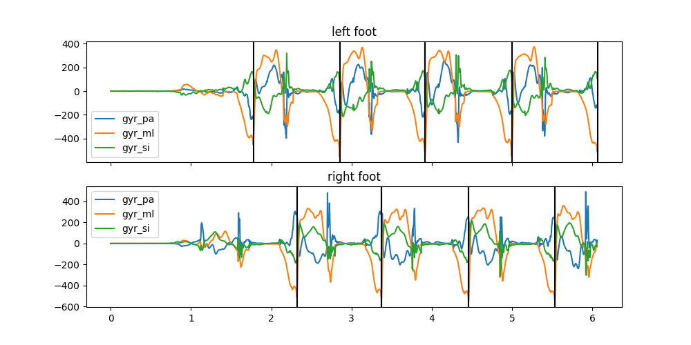
fig, axs = plt.subplots(nrows=2, figsize=(10, 5), sharex=True)
for ax, foot in zip(axs, ["left", "right"]):
    ax.set_title(f"{foot} foot")
    convert_left_foot_to_fbf(template_data[f"{foot}_sensor"])[BF_GYR].plot(ax=ax)
    # Mark stride borders with vertical lines
    for _i, val in template_stride_borders[f"{foot}_sensor"].iterrows():
        ax.axvline(x=val["end"] / sampling_rate_hz, color="k")
        ax.axvline(x=val["start"] / sampling_rate_hz, color="k")

plt.show()
Creating a custom template#
Based on the stride borders in the selected data, we can create a custom template.
First we need to extract the data of the individual strides.
We can do that using the iterate_region_data helper.
Note this helper returns a generator that yields the data of the individual strides.
from gaitmap.utils.array_handling import iterate_region_data

# Convert data to body frame
bf_template_data = convert_to_fbf(template_data, left_like="left_", right_like="right_")

# Split the data of the left and the right foot to use it independently
bf_template_data_list = to_dict_multi_sensor_data(bf_template_data).values()
stride_generator = iterate_region_data(bf_template_data_list, template_stride_borders.values())

next(stride_generator)
We recreate the generator, as the next call above removed the first stride
stride_generator = iterate_region_data(bf_template_data_list, template_stride_borders.values())
Interpolating the template data#
There are multiple ways to turn the data of the individual strides into a template. The method that is implemented in gaitmap interpolates all strides to the same length and then averages the data sample by sample.
To use this method we need to create an instance of the InterpolatedDtwTemplate
class.
from gaitmap.stride_segmentation import InterpolatedDtwTemplate

template = InterpolatedDtwTemplate()  # For now we do not change the arguments and keep everything as default
With this template we can call self_optimize with our strides to create a template based on linear interpolation.
The final template length will be the average length of the individual strides.
template.self_optimize(stride_generator, sampling_rate_hz, columns=BF_GYR)

template.get_data().plot()
plt.show()
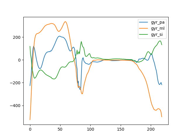
As you can see, this template represents an average stride.
While we could use this template as-is, usually it makes sense to normalize the template. This will result in more comparable cost values of the DTW and allows us to adjust the template for different data ranges. For that we need to provide a scaling method. The template will store the scaling method, so that we can apply the same scaling to the data.
Here, we need to make a choice, if we want to apply the exact same scaling factors of the template to the data, or just the same method of scaling. To understand the difference, let’s do both
Same scaling factors#
from gaitmap.data_transform import StandardScaler, TrainableStandardScaler

template = InterpolatedDtwTemplate(scaling=TrainableStandardScaler())

stride_generator = iterate_region_data(bf_template_data_list, template_stride_borders.values())
template.self_optimize(stride_generator, sampling_rate_hz, columns=BF_GYR)
InterpolatedDtwTemplate(data=         gyr_pa      gyr_ml      gyr_si
0   -225.617192 -524.765957  117.965788
1   -183.727973 -441.137654   43.403129
2   -137.772901 -317.382564   12.556771
3    -42.393835 -193.704262  -51.763276
4     45.719194  -81.699326  -89.331217
..          ...         ...         ...
214 -216.232104 -430.958697  163.367427
215 -215.160208 -435.032678  166.323753
216 -204.476716 -443.916617  165.512217
217 -198.979137 -460.683229  153.859775
218 -217.537175 -499.283456  132.857482

[219 rows x 3 columns], interpolation_method='linear', n_samples=None, sampling_rate_hz=204.8, scaling=TrainableStandardScaler(ddof=1, mean=-2.228665883735075, std=145.51707439675124), use_cols=None)
After the template is created, we can see that the data we get from get_data is normalized and the scaler we
provided holds the mean and standard deviation of the template.
template.get_data().plot()
plt.show()
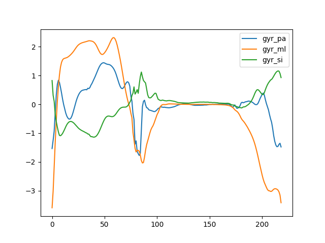
TrainableStandardScaler(ddof=1, mean=-2.228665883735075, std=145.51707439675124)
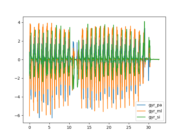
We can apply the scaling to other data using the transform_data method.
This uses exactly the same scaling factors as the template.
template.transform_data(bf_data, sampling_rate_hz=sampling_rate_hz)["left_sensor"][BF_GYR].plot()
plt.show()

Same method, but with the same scaling factors#
Alternatively, we can use the same scaling method as the template, but let the method recalculate the scaling factors. For this, we use the non-trainable version of the scaler. This will not store the scaling factors, but will apply standard scaling on the template and the data independently.
template = InterpolatedDtwTemplate(scaling=StandardScaler())

stride_generator = iterate_region_data(bf_template_data_list, template_stride_borders.values())
template.self_optimize(stride_generator, sampling_rate_hz, columns=BF_GYR)

template.get_data().plot()
plt.show()

The template data still looks identical, but the scaled data is slightly different, as the mean and the std of the data is used instead of the template.
template.transform_data(bf_data, sampling_rate_hz=sampling_rate_hz)["left_sensor"][BF_GYR].plot()
plt.show()
Which approach you should use depends on the application. If you expect the matching data to have the same data range as the template, it makes sense to only learn the factors once. However, if you expect the data to have a different data range, you should scale the data independently. However, this might result in issues, if the normalization/scaling method amplifies data noise.
For now we will switch back to a simple scaler trained on the template data and then show how to apply the template.
from gaitmap.data_transform import TrainableAbsMaxScaler

template = InterpolatedDtwTemplate(scaling=TrainableAbsMaxScaler())

stride_generator = iterate_region_data(bf_template_data_list, template_stride_borders.values())
template.self_optimize(stride_generator, sampling_rate_hz, columns=BF_GYR)
InterpolatedDtwTemplate(data=         gyr_pa      gyr_ml      gyr_si
0   -225.617192 -524.765957  117.965788
1   -183.727973 -441.137654   43.403129
2   -137.772901 -317.382564   12.556771
3    -42.393835 -193.704262  -51.763276
4     45.719194  -81.699326  -89.331217
..          ...         ...         ...
214 -216.232104 -430.958697  163.367427
215 -215.160208 -435.032678  166.323753
216 -204.476716 -443.916617  165.512217
217 -198.979137 -460.683229  153.859775
218 -217.537175 -499.283456  132.857482

[219 rows x 3 columns], interpolation_method='linear', n_samples=None, sampling_rate_hz=204.8, scaling=TrainableAbsMaxScaler(data_max=524.7659568483249, out_max=1), use_cols=None)
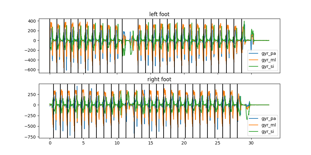
Apply the template to the data#
Now we can apply the template to the data using the normal BarthDtw method.
Note, that all Dtw methods apply the data transform internally, so we do not need to transform the data before we
apply the template.
from gaitmap.stride_segmentation import BarthDtw

dtw = BarthDtw(template=template)
dtw.segment(bf_data, sampling_rate_hz=sampling_rate_hz)

fig, axs = plt.subplots(nrows=2, figsize=(10, 5), sharex=True)
for ax, foot in zip(axs, ["left", "right"]):
    ax.set_title(f"{foot} foot")
    bf_data[f"{foot}_sensor"][BF_GYR].plot(ax=ax)
    # Mark stride borders with vertical lines
    for _i, val in dtw.stride_list_[f"{foot}_sensor"].iterrows():
        ax.axvline(x=val["end"] / sampling_rate_hz, color="k")
        ax.axvline(x=val["start"] / sampling_rate_hz, color="k")

plt.show()

# # sphinx_gallery_thumbnail_number = 2
Total running time of the script: ( 0 minutes 7.144 seconds)
Estimated memory usage: 44 MB