Note
Click here to download the full example code
HMM stride segmentation - Prediction with pre-trained model#
This example illustrates how a Hidden Markov Model (HMM) implemented by the
HmmStrideSegmentation can be used to detect strides in a continuous signal of
an IMU signal.
The used implementation is based on the work of Roth et al [1]
import matplotlib.pyplot as plt
import numpy as np

np.random.seed(0)
Getting some example data#
For this we take some example data that contains the regular walking movement during a 2x20m walk test of a healthy subject. The IMU signals are already rotated so that they align with the gaitmap SF coordinate system. The data contains information from two sensors - one from the right and one from the left foot.
from gaitmap.example_data import get_healthy_example_imu_data

data = get_healthy_example_imu_data()
sampling_rate_hz = 204.8
data.sort_index(axis=1).head(1)
Preparing the data#
The HMM only makes use of the gyro information. Further, if you use this model, your data is expected to be in the gaitmap body-frame to be able to use the same model for the left and the right foot. Therefore, we need to transform the dataset into the body frame.
from gaitmap.utils.coordinate_conversion import convert_to_fbf

# We use the `..._like` parameters to identify the data of the left and the right foot based on the name of the sensor.
bf_data = convert_to_fbf(data, left_like="left_", right_like="right_")
Selecting a pre-trained model#
This library ships with pre-trained models that can be directly used for prediction/ segmentation. It is generated based on manually segmented strides from healthy participants and PD patients. We can load the model a look at some of its parameters
from gaitmap.stride_segmentation.hmm import PreTrainedRothSegmentationModel

roth_hmm_model = PreTrainedRothSegmentationModel()

print(f"Number of states, stride-model: {roth_hmm_model.stride_model.n_states:d}")
print(f"Number of states, transition-model: {roth_hmm_model.transition_model.n_states:d}")
np.set_printoptions(precision=3, linewidth=180, suppress=True)
print(f"Transition matrix:\n{roth_hmm_model.model.dense_transition_matrix()[0:-2, 0:-2]}")
Number of states, stride-model: 20
Number of states, transition-model: 5
Transition matrix:
[[0.882 0.036 0.    0.054 0.    0.028 0.    0.    0.    0.    0.    0.    0.    0.    0.    0.    0.    0.    0.    0.    0.    0.    0.    0.    0.   ]
 [0.    0.975 0.025 0.    0.    0.    0.    0.    0.    0.    0.    0.    0.    0.    0.    0.    0.    0.    0.    0.    0.    0.    0.    0.    0.   ]
 [0.    0.    0.975 0.025 0.    0.    0.    0.    0.    0.    0.    0.    0.    0.    0.    0.    0.    0.    0.    0.    0.    0.    0.    0.    0.   ]
 [0.    0.    0.    0.942 0.058 0.    0.    0.    0.    0.    0.    0.    0.    0.    0.    0.    0.    0.    0.    0.    0.    0.    0.    0.    0.   ]
 [0.085 0.    0.    0.    0.915 0.    0.    0.    0.    0.    0.    0.    0.    0.    0.    0.    0.    0.    0.    0.    0.    0.    0.    0.    0.   ]
 [0.    0.    0.    0.    0.    0.589 0.411 0.    0.    0.    0.    0.    0.    0.    0.    0.    0.    0.    0.    0.    0.    0.    0.    0.    0.   ]
 [0.    0.    0.    0.    0.    0.    0.667 0.333 0.    0.    0.    0.    0.    0.    0.    0.    0.    0.    0.    0.    0.    0.    0.    0.    0.   ]
 [0.    0.    0.    0.    0.    0.    0.    0.68  0.32  0.    0.    0.    0.    0.    0.    0.    0.    0.    0.    0.    0.    0.    0.    0.    0.   ]
 [0.    0.    0.    0.    0.    0.    0.    0.    0.694 0.306 0.    0.    0.    0.    0.    0.    0.    0.    0.    0.    0.    0.    0.    0.    0.   ]
 [0.    0.    0.    0.    0.    0.    0.    0.    0.    0.696 0.304 0.    0.    0.    0.    0.    0.    0.    0.    0.    0.    0.    0.    0.    0.   ]
 [0.    0.    0.    0.    0.    0.    0.    0.    0.    0.    0.68  0.32  0.    0.    0.    0.    0.    0.    0.    0.    0.    0.    0.    0.    0.   ]
 [0.    0.    0.    0.    0.    0.    0.    0.    0.    0.    0.    0.691 0.309 0.    0.    0.    0.    0.    0.    0.    0.    0.    0.    0.    0.   ]
 [0.    0.    0.    0.    0.    0.    0.    0.    0.    0.    0.    0.    0.682 0.318 0.    0.    0.    0.    0.    0.    0.    0.    0.    0.    0.   ]
 [0.    0.    0.    0.    0.    0.    0.    0.    0.    0.    0.    0.    0.    0.653 0.347 0.    0.    0.    0.    0.    0.    0.    0.    0.    0.   ]
 [0.    0.    0.    0.    0.    0.    0.    0.    0.    0.    0.    0.    0.    0.    0.674 0.326 0.    0.    0.    0.    0.    0.    0.    0.    0.   ]
 [0.    0.    0.    0.    0.    0.    0.    0.    0.    0.    0.    0.    0.    0.    0.    0.69  0.31  0.    0.    0.    0.    0.    0.    0.    0.   ]
 [0.    0.    0.    0.    0.    0.    0.    0.    0.    0.    0.    0.    0.    0.    0.    0.    0.668 0.332 0.    0.    0.    0.    0.    0.    0.   ]
 [0.    0.    0.    0.    0.    0.    0.    0.    0.    0.    0.    0.    0.    0.    0.    0.    0.    0.764 0.236 0.    0.    0.    0.    0.    0.   ]
 [0.    0.    0.    0.    0.    0.    0.    0.    0.    0.    0.    0.    0.    0.    0.    0.    0.    0.    0.849 0.151 0.    0.    0.    0.    0.   ]
 [0.    0.    0.    0.    0.    0.    0.    0.    0.    0.    0.    0.    0.    0.    0.    0.    0.    0.    0.    0.765 0.235 0.    0.    0.    0.   ]
 [0.    0.    0.    0.    0.    0.    0.    0.    0.    0.    0.    0.    0.    0.    0.    0.    0.    0.    0.    0.    0.632 0.368 0.    0.    0.   ]
 [0.    0.    0.    0.    0.    0.    0.    0.    0.    0.    0.    0.    0.    0.    0.    0.    0.    0.    0.    0.    0.    0.594 0.406 0.    0.   ]
 [0.    0.    0.    0.    0.    0.    0.    0.    0.    0.    0.    0.    0.    0.    0.    0.    0.    0.    0.    0.    0.    0.    0.564 0.436 0.   ]
 [0.    0.    0.    0.    0.    0.    0.    0.    0.    0.    0.    0.    0.    0.    0.    0.    0.    0.    0.    0.    0.    0.    0.    0.398 0.602]
 [0.039 0.    0.    0.    0.    0.369 0.    0.    0.    0.    0.    0.    0.    0.    0.    0.    0.    0.    0.    0.    0.    0.    0.    0.    0.592]]
Inspecting the results#
The main output is the stride_list_, which contains the start and the end of all identified strides.
As we passed a dataset with two sensors, the output will be a dictionary.
stride_list_left = hmm_seg.stride_list_["left_sensor"]
print(f"{len(stride_list_left)} strides were detected.")
stride_list_left.head()
29 strides were detected.
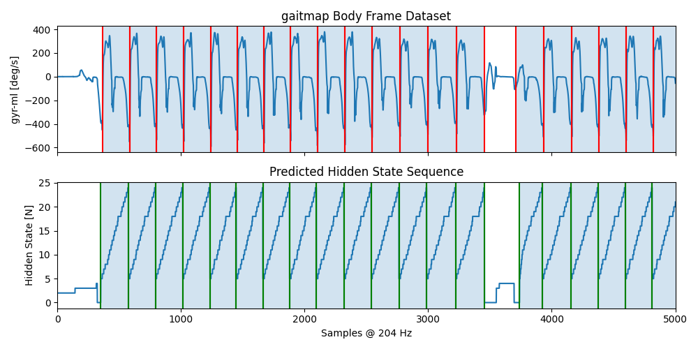
To get a better understanding of the results, we can plot additional information about the results.
The top row shows the gyr_ml axis with the segmented strides plotted on top.
They are postprocessed to snap to the closed data minimum.
In the second row the predicted hidden state sequence of the HMM is plotted (this is the transformed version, matching
the input signal).
Each transition from the last (n=25) to the first (n=5) stride state marks a potential start/end of a stride.
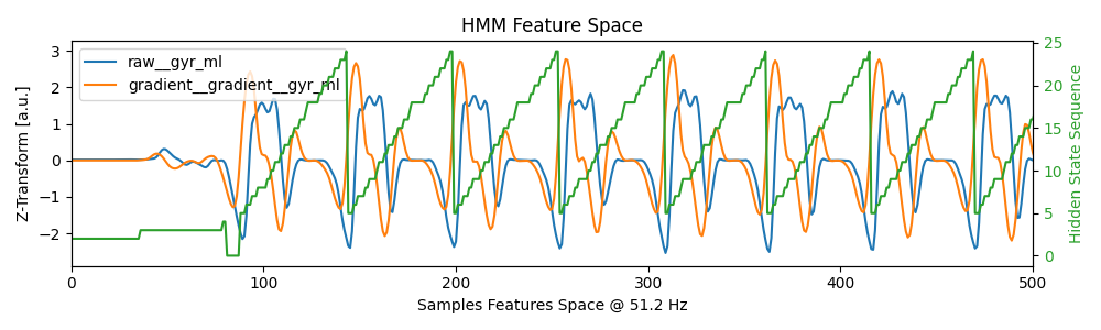
The second plot shows the results in the feature space (which will depend on the feature space setting during the
training step).
Here this is a downsampled and filtered representative of the gyr_ml signal as well as its window based gradient.
All features are z-transformed (note we z-transform the new data independently from the training data).
Again, the predicted hidden state sequence is plotted together with the data.
Only the first couple of strides of the left foot are shown.
sensor = "left_sensor"

fig, axs = plt.subplots(nrows=2, sharex=True, figsize=(10, 5))
axs[0].set_title("gaitmap Body Frame Dataset")
axs[0].plot(bf_data.reset_index(drop=True)[sensor]["gyr_ml"])
for start, end in hmm_seg.stride_list_["left_sensor"].to_numpy():
    axs[0].axvline(start, c="r")
    axs[0].axvline(end, c="r")
    axs[0].axvspan(start, end, alpha=0.2)
axs[0].set_ylabel("gyr-ml [deg/s]")

axs[1].set_title("Predicted Hidden State Sequence")
axs[1].plot(hmm_seg.hidden_state_sequence_[sensor])
for start, end in hmm_seg.matches_start_end_original_[sensor]:
    axs[1].axvline(start, c="g")
    axs[1].axvline(end, c="g")
    axs[1].axvspan(start, end, alpha=0.2)
axs[1].set_ylabel("Hidden State [N]")

axs[1].set_xlabel("Samples @ %d Hz" % sampling_rate_hz)
plt.xlim([0, 5000])
fig.tight_layout()
plt.show()

fig, ax1 = plt.subplots(figsize=(10, 3))
plt.title("HMM Feature Space")
ax1.set_xlabel(f"Samples Features Space @ {hmm_seg.model.feature_transform.sampling_rate_feature_space_hz} Hz")
ax1.set_ylabel("Z-Transform [a.u.]")
feature_space_date = hmm_seg.result_model_[sensor].feature_space_data_
ax1.plot(feature_space_date)
ax1.legend(feature_space_date.columns.to_list())

ax2 = ax1.twinx()
ax2.set_ylabel("Hidden State Sequence", color="tab:green")
hidden_state_sequence_feature_space = hmm_seg.result_model_[sensor].hidden_state_sequence_feature_space_
ax2.plot(hidden_state_sequence_feature_space, color="tab:green")
ax2.tick_params(axis="y", labelcolor="tab:green")

plt.xlim([0, 500])
fig.tight_layout()
plt.show()
Total running time of the script: ( 0 minutes 3.128 seconds)
Estimated memory usage: 11 MB