Ullrich gait sequence detection#

This example illustrates how the gait sequence detection by the UllrichGaitSequenceDetection can be used to detect gait sequences within an IMU signal stream. The used implementation is based on the work of Ullrich et al. [1]. The underlying algorithm works under the assumption that the IMU gait signal shows a characteristic pattern of harmonics when looking at the power spectral density. This is in contrast to cyclic non-gait signals, where there is usually only one dominant frequency present.

Getting some example data#

For this we take some example data that contains the regular walking movement during a 2x20m walk test of a healthy subject. The IMU signals are already rotated so that they align with the gaitmap SF coordinate system. The data contains information from two sensors - one from the right and one from the left foot. For further information regarding the coordinate system refer to the coordinate system guide.

from gaitmap.example_data import get_healthy_example_imu_data

data = get_healthy_example_imu_data()
sampling_rate_hz = 204.8
data.sort_index(axis=1).head(1)

sensor	left_sensor						right_sensor
axis	acc_x	acc_y	acc_z	gyr_x	gyr_y	gyr_z	acc_x	acc_y	acc_z	gyr_x	gyr_y	gyr_z
0.0	0.880811	2.762208	9.40865	-0.112402	-0.032157	-0.062261	0.311553	-2.398646	9.513275	-0.323037	0.084604	-0.025288

Preparing the data#

The data is expected to be in the gaitmap BF to be able to use the same template for the left and the right foot. Therefore, we need to transform the dataset into the body frame. For further information regarding the coordinate system refer to the coordinate system guide.

from gaitmap.utils.coordinate_conversion import convert_to_fbf

# We use the `..._like` parameters to identify the data of the left and the right foot based on the name of the sensor.
bf_data = convert_to_fbf(data, left_like="left_", right_like="right_")

# for demonstration purposes we will for now stick with the data of one foot only
bf_data = bf_data["left_sensor"]

import numpy as np

Add rest and non-gait data#

Additionally to the gait data we use some artificial signal to simulate rest and an arbitrary cyclic but non-gait movement.

import pandas as pd

# use zeros for rest
rest_df = pd.DataFrame([[0] * bf_data.shape[1]], columns=bf_data.columns)
rest_df = pd.concat([rest_df] * 2048)

# create a sine signal to mimic non-gait
samples = 2048
t = np.arange(samples) / sampling_rate_hz
freq = 1
test_signal = np.sin(2 * np.pi * freq * t) * 200
test_signal_reshaped = np.tile(test_signal, (bf_data.shape[1], 1)).T
non_gait_df = pd.DataFrame(test_signal_reshaped, columns=bf_data.columns)

# combine rest, gait and non-gait data to one dataframe
test_data_df = pd.concat([rest_df, bf_data, rest_df, non_gait_df, rest_df, bf_data, rest_df], ignore_index=True)
test_data_df.head(1)

	acc_pa	acc_ml	acc_si	gyr_pa	gyr_ml	gyr_si
0	0.0	0.0	0.0	0.0	0.0	0.0

Applying the gait sequence detection#

First we need to initialize the Ullrich gait sequence detection. In most cases it is sufficient to keep all parameters at default. These are set as presented in the original paper. In correspondence with the original publication usually the gyr_ml signal is investigated regarding the presence of gait. It is however also possible to use gyr or acc in order to apply the algorithm to the signal norm of gyroscope or accelerometer, respectively. Furthermore the acc_si was investigated in the paper. The optimal value for the peak_prominence which serves as a threshold for the harmonic frequency peaks was found to be 17 in the publication for the gyr_ml setting. All experiments in the paper were performed with a window_size_s of 10 s, where subsequent windows were overlapping by 50%. The default value for the active_signal_threshold was found experimentally and is per default set to 50 deg/s for the usage of gyr_ml. The algorithm first identifies the dominant frequency of the signal window, which should usually be within the locomotion_band of (0.5 3) Hz. For very slow gait, the lower bound may have to be decreased.

from gaitmap.gait_detection import UllrichGaitSequenceDetection

gsd = UllrichGaitSequenceDetection()
gsd = gsd.detect(data=test_data_df, sampling_rate_hz=sampling_rate_hz)

/home/docs/checkouts/readthedocs.org/user_builds/gaitmap/checkouts/v2.6.0/packages/gaitmap_mad/src/gaitmap_mad/gait_detection/_ullrich_gait_sequence_detection.py:384: PeakPropertyWarning: some peaks have a prominence of 0
  peak_prominence = peak_prominences(f_s_1d_flat, closest_peaks)[0].reshape(harmonics_candidates.shape)

Inspecting the results#

The main output is gait_sequences_, which is a RegionsOfInterestList that contains the samples of start and end of all detected gait sequences. It furthermore has a column gs_id for the gait sequence id which is used in further processing steps to assign for example single strides to their respective gs_id.

gait_sequences = gsd.gait_sequences_
print(f"{len(gait_sequences)} gait sequences were detected.")
gait_sequences.head()

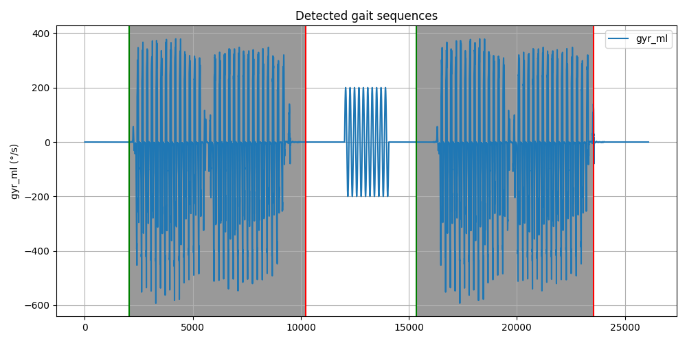
2 gait sequences were detected.

	gs_id	start	end
0	0	2048	10240
1	1	15360	23552

To get a better understanding of the results, we can plot the data and the gait detected gait sequences. The vertical lines show the start and end of the gait sequences.

import matplotlib.pyplot as plt

fig, ax1 = plt.subplots(1, sharex=True, figsize=(10, 5))
ax1.plot(test_data_df["gyr_ml"], label="gyr_ml")

start_idx = gait_sequences["start"].to_numpy().astype(int)
end_idx = gait_sequences["end"].to_numpy().astype(int)

for _i, gs in gait_sequences.iterrows():
    start_sample = int(gs["start"])
    end_sample = int(gs["end"])
    ax1.axvline(start_sample, color="g")
    ax1.axvline(end_sample, color="r")
    ax1.axvspan(start_sample, end_sample, facecolor="grey", alpha=0.8)

ax1.grid(True)

ax1.set_title("Detected gait sequences")
ax1.set_ylabel("gyr_ml (°/s)")
plt.legend(loc="best")

fig.tight_layout()
fig.show()

Total running time of the script: ( 0 minutes 5.353 seconds)

Estimated memory usage: 11 MB

Gallery generated by Sphinx-Gallery