Note
Click here to download the full example code
SegmentationModel Training#
This example illustrates how a Hidden Markov Model (HMM) implemented by the
RothSegmentationHmm can be trained from IMU data and presegmented stride lists.
The used implementation is based on the work of Roth et al [1]
import numpy as np
from matplotlib import pyplot as plt

np.random.seed(1)
Getting some example data#
For this we take some example data that contains the regular walking movement during a 2x20m walk test of a healthy subject. The IMU signals are already rotated so that they align with the gaitmap SF coordinate system. The data contains information from two sensors - one from the right and one from the left foot.
from gaitmap.example_data import get_healthy_example_imu_data

data = get_healthy_example_imu_data()
sampling_rate_hz = 204.8
data.sort_index(axis=1).head(1)
Preparing the data#
The HMM only makes use of the gyro information. Further, if you use this model, your data is expected to be in the gaitmap body-frame to be able to use the same model for the left and the right foot. Therefore, we need to transform the dataset into the body frame.
from gaitmap.utils.coordinate_conversion import convert_to_fbf

# We use the `..._like` parameters to identify the data of the left and the right foot based on the name of the sensor.
bf_data = convert_to_fbf(data, left_like="left_", right_like="right_")
Getting the example stride list#
For this we take the ground truth stride list provided with the example data.
For new data this stride list can be generated by running the algorithms provided in the
stride_segmentation module and then manually corrected, or by creating a stride list using ground
truth data.
from gaitmap.example_data import get_healthy_example_stride_borders

stride_list = get_healthy_example_stride_borders()

from gaitmap.data_transform import ButterworthFilter
Initialize Model Parameters - Feature Transformation#
Here we define the feature space in which model training and later prediction will take place. You can choose different axis and or feature combinations as well as downsampling, filter and standardization steps. The following example has proved to work well in most cases.
from gaitmap.stride_segmentation.hmm import RothHmmFeatureTransformer

feature_transform = RothHmmFeatureTransformer(
    sampling_rate_feature_space_hz=51.2,
    axes=["gyr_ml"],
    features=["raw", "gradient"],
    low_pass_filter=ButterworthFilter(order=4, cutoff_freq_hz=10),
    window_size_s=0.2,
    standardization=True,
)
Initialize Model Parameters - Sub HMMs#
The segmentation process is defined as a two-class problem, namely “strides” and “transitions/null”. For each class we define a separate HMM and define all its components. Notice that the stride and transition model are different in architecture, number of states or number of gaussian mixture model (GMM) components. In this example all configurable parameters are exposed. These parameters might require optimization for your specific type of dataset!
from gaitmap.stride_segmentation.hmm import SimpleHmm

stride_model = SimpleHmm(
    n_states=20,
    n_gmm_components=6,
    algo_train="baum-welch",
    stop_threshold=1e-9,
    max_iterations=5,
    architecture="left-right-strict",
    verbose=True,
    name="stride_model",
)

transition_model = SimpleHmm(
    n_states=5,
    n_gmm_components=3,
    algo_train="baum-welch",
    stop_threshold=1e-9,
    max_iterations=5,
    architecture="left-right-loose",
    verbose=True,
    name="transition_model",
)
Initialize Model Parameters - Segmentation Model#
Finally we can combine the feature extraction and our defined sub-HMMs to the actual segmentation model were we can invoke the training process. Again, all configurable parameters are exposed for demonstration purpose. These parameters should again work for most usecases.
from gaitmap.stride_segmentation.hmm import RothSegmentationHmm

segmentation_model = RothSegmentationHmm(
    stride_model=stride_model,
    transition_model=transition_model,
    feature_transform=feature_transform,
    algo_predict="viterbi",
    algo_train="baum-welch",
    stop_threshold=1e-9,
    max_iterations=1,
    initialization="labels",
    verbose=True,
    name="segmentation_model",
)
Prepare Data for Training#
The HMM does not differentiate between left or right strides, (this is why we must have our data in the body-frame convention!). The main input format for the training process are gait sequences which include transitions as well as valid strides. To train on multiple sequences, we can just feed a list of gaitsequences into the model for training. For each gait sequence we also need to have a valid stride list. In this example we handle the data from the left and right foot as separate gait sequences and add them to a simple list. We have to do the same for the stride lists.
data_train_sequence = [bf_data["left_sensor"], bf_data["right_sensor"]]
stride_list_sequence = [stride_list["left_sensor"], stride_list["right_sensor"]]
Training#
Finally! Sit back relax and let the magic happen (depending on the number of input sequences this can take up to >30min). However, this small example runs quite fast! The model will internally perform the feature transformation of the dataset, train the individual sub models and finally combine them to a flatted segmentation model.
segmentation_model = segmentation_model.self_optimize(
    data_train_sequence, stride_list_sequence, sampling_rate_hz=sampling_rate_hz
)
[1] Improvement: 341.2437178557084      Time (s): 0.2085
[2] Improvement: 109.29279107726325     Time (s): 0.2077
[3] Improvement: 25.279694613596803     Time (s): 0.2082
[4] Improvement: 52.723999946801996     Time (s): 0.2078
[5] Improvement: -3.5209243279850853    Time (s): 0.2088
Total Training Improvement: 525.0192791653853
Total Training Time (s): 1.2424
/home/docs/checkouts/readthedocs.org/user_builds/gaitmap/checkouts/v2.6.0/packages/gaitmap_mad/src/gaitmap_mad/stride_segmentation/hmm/_utils.py:333: UserWarning: During training the improvement per epoch became NaN/infinite or negative! Run `self_optimize_with_info` and inspect the history element for more information. With a high likelihood, the final model is not usable and will result in errors during prediction. This usually happens when there is not enough data for a large number of distributions and states. To avoid this issue, reduce the number of distributions per state or the number of states. Or ideally, provide more data.
  warnings.warn(
[1] Improvement: 723.4614150029679      Time (s): 0.008724
[2] Improvement: 62.761125573766094     Time (s): 0.009014
[3] Improvement: 28.507724633026555     Time (s): 0.009044
[4] Improvement: 16.114249821317117     Time (s): 0.008944
[5] Improvement: 33.07876970054485      Time (s): 0.00881
Total Training Improvement: 863.9232847316225
Total Training Time (s): 0.0545
[1] Improvement: 43.84714447262195      Time (s): 0.2094
Total Training Improvement: 43.84714447262195
Total Training Time (s): 0.4585
Inspecting the Results#
Now all internal models which were initialized as “None” should be populated by pomegranate models. We can now have a look at the final transition matrix or the trained distributions (GMMs). You could now either use the model to predict stride borders on an unseen sequence or save it to a json file for later use.
np.set_printoptions(precision=3, linewidth=180, suppress=True)

print(segmentation_model.model.dense_transition_matrix()[0:-2, 0:-2])

print(segmentation_model.model.states[10])
[[0.891 0.109 0.    0.    0.    0.    0.    0.    0.    0.    0.    0.    0.    0.    0.    0.    0.    0.    0.    0.    0.    0.    0.    0.    0.   ]
 [0.    0.925 0.075 0.    0.    0.    0.    0.    0.    0.    0.    0.    0.    0.    0.    0.    0.    0.    0.    0.    0.    0.    0.    0.    0.   ]
 [0.    0.    0.86  0.14  0.    0.    0.    0.    0.    0.    0.    0.    0.    0.    0.    0.    0.    0.    0.    0.    0.    0.    0.    0.    0.   ]
 [0.    0.    0.    0.949 0.051 0.    0.    0.    0.    0.    0.    0.    0.    0.    0.    0.    0.    0.    0.    0.    0.    0.    0.    0.    0.   ]
 [0.158 0.    0.    0.    0.795 0.047 0.    0.    0.    0.    0.    0.    0.    0.    0.    0.    0.    0.    0.    0.    0.    0.    0.    0.    0.   ]
 [0.    0.    0.    0.    0.    0.667 0.333 0.    0.    0.    0.    0.    0.    0.    0.    0.    0.    0.    0.    0.    0.    0.    0.    0.    0.   ]
 [0.    0.    0.    0.    0.    0.    0.669 0.331 0.    0.    0.    0.    0.    0.    0.    0.    0.    0.    0.    0.    0.    0.    0.    0.    0.   ]
 [0.    0.    0.    0.    0.    0.    0.    0.627 0.373 0.    0.    0.    0.    0.    0.    0.    0.    0.    0.    0.    0.    0.    0.    0.    0.   ]
 [0.    0.    0.    0.    0.    0.    0.    0.    0.716 0.284 0.    0.    0.    0.    0.    0.    0.    0.    0.    0.    0.    0.    0.    0.    0.   ]
 [0.    0.    0.    0.    0.    0.    0.    0.    0.    0.664 0.336 0.    0.    0.    0.    0.    0.    0.    0.    0.    0.    0.    0.    0.    0.   ]
 [0.    0.    0.    0.    0.    0.    0.    0.    0.    0.    0.666 0.334 0.    0.    0.    0.    0.    0.    0.    0.    0.    0.    0.    0.    0.   ]
 [0.    0.    0.    0.    0.    0.    0.    0.    0.    0.    0.    0.652 0.348 0.    0.    0.    0.    0.    0.    0.    0.    0.    0.    0.    0.   ]
 [0.    0.    0.    0.    0.    0.    0.    0.    0.    0.    0.    0.    0.589 0.411 0.    0.    0.    0.    0.    0.    0.    0.    0.    0.    0.   ]
 [0.    0.    0.    0.    0.    0.    0.    0.    0.    0.    0.    0.    0.    0.516 0.484 0.    0.    0.    0.    0.    0.    0.    0.    0.    0.   ]
 [0.    0.    0.    0.    0.    0.    0.    0.    0.    0.    0.    0.    0.    0.    0.527 0.473 0.    0.    0.    0.    0.    0.    0.    0.    0.   ]
 [0.    0.    0.    0.    0.    0.    0.    0.    0.    0.    0.    0.    0.    0.    0.    0.525 0.475 0.    0.    0.    0.    0.    0.    0.    0.   ]
 [0.    0.    0.    0.    0.    0.    0.    0.    0.    0.    0.    0.    0.    0.    0.    0.    0.447 0.553 0.    0.    0.    0.    0.    0.    0.   ]
 [0.    0.    0.    0.    0.    0.    0.    0.    0.    0.    0.    0.    0.    0.    0.    0.    0.    0.632 0.368 0.    0.    0.    0.    0.    0.   ]
 [0.    0.    0.    0.    0.    0.    0.    0.    0.    0.    0.    0.    0.    0.    0.    0.    0.    0.    0.82  0.18  0.    0.    0.    0.    0.   ]
 [0.    0.    0.    0.    0.    0.    0.    0.    0.    0.    0.    0.    0.    0.    0.    0.    0.    0.    0.    0.494 0.506 0.    0.    0.    0.   ]
 [0.    0.    0.    0.    0.    0.    0.    0.    0.    0.    0.    0.    0.    0.    0.    0.    0.    0.    0.    0.    0.618 0.382 0.    0.    0.   ]
 [0.    0.    0.    0.    0.    0.    0.    0.    0.    0.    0.    0.    0.    0.    0.    0.    0.    0.    0.    0.    0.    0.67  0.33  0.    0.   ]
 [0.    0.    0.    0.    0.    0.    0.    0.    0.    0.    0.    0.    0.    0.    0.    0.    0.    0.    0.    0.    0.    0.    0.647 0.353 0.   ]
 [0.    0.    0.    0.    0.    0.    0.    0.    0.    0.    0.    0.    0.    0.    0.    0.    0.    0.    0.    0.    0.    0.    0.    0.645 0.355]
 [0.017 0.    0.    0.    0.    0.304 0.    0.    0.    0.    0.    0.    0.    0.    0.    0.    0.    0.    0.    0.    0.    0.    0.    0.    0.68 ]]
{
    "class" : "State",
    "distribution" : {
        "class" : "GeneralMixtureModel",
        "distributions" : [
            {
                "class" : "Distribution",
                "name" : "MultivariateGaussianDistribution",
                "parameters" : [
                    [
                        1.5126628727953728,
                        -1.2325509070704483
                    ],
                    [
                        [
                            0.005687593991405892,
                            0.0023472485533848997
                        ],
                        [
                            0.0023472485533848997,
                            0.040877832841576395
                        ]
                    ]
                ],
                "frozen" : false
            },
            {
                "class" : "Distribution",
                "name" : "MultivariateGaussianDistribution",
                "parameters" : [
                    [
                        1.246494912094264,
                        -1.5631885798768912
                    ],
                    [
                        [
                            0.02247323938290144,
                            0.00967374480066069
                        ],
                        [
                            0.00967374480066069,
                            0.04359681875993598
                        ]
                    ]
                ],
                "frozen" : false
            },
            {
                "class" : "Distribution",
                "name" : "MultivariateGaussianDistribution",
                "parameters" : [
                    [
                        -0.14468908268310057,
                        -0.32692151837939903
                    ],
                    [
                        [
                            0.004734574595004851,
                            -0.007669695586920108
                        ],
                        [
                            -0.007669695586920108,
                            0.01245693964354575
                        ]
                    ]
                ],
                "frozen" : false
            },
            {
                "class" : "Distribution",
                "name" : "MultivariateGaussianDistribution",
                "parameters" : [
                    [
                        1.7391578250883177,
                        -1.4912029930432096
                    ],
                    [
                        [
                            0.0011035263021169747,
                            0.002104007563097542
                        ],
                        [
                            0.002104007563097542,
                            0.0349554610296975
                        ]
                    ]
                ],
                "frozen" : false
            },
            {
                "class" : "Distribution",
                "name" : "MultivariateGaussianDistribution",
                "parameters" : [
                    [
                        1.1445625377737405,
                        -1.7356582771533349
                    ],
                    [
                        [
                            0.015585621689172442,
                            -0.01362748197089966
                        ],
                        [
                            -0.01362748197089966,
                            0.031239367536969237
                        ]
                    ]
                ],
                "frozen" : false
            },
            {
                "class" : "Distribution",
                "name" : "MultivariateGaussianDistribution",
                "parameters" : [
                    [
                        0.7189351972580712,
                        -1.886781134785975
                    ],
                    [
                        [
                            0.02468903546241029,
                            0.00967892554067703
                        ],
                        [
                            0.00967892554067703,
                            0.02033165397565948
                        ]
                    ]
                ],
                "frozen" : false
            }
        ],
        "weights" : [
            0.30984372119247067,
            0.27134257464797806,
            0.01725767107205237,
            0.041169920711634715,
            0.09302063408620882,
            0.2673654782896554
        ]
    },
    "name" : "sa",
    "weight" : 1.0
}
Applying the Model to a Sequence#
in the follwoing we will apply the model to the same sequence we used for training, just to show that the model “learned” something. We will also plot the results to see how well the model performs.
from gaitmap.stride_segmentation.hmm import HmmStrideSegmentation

hmm = HmmStrideSegmentation(segmentation_model).segment(bf_data, sampling_rate_hz=sampling_rate_hz)
hmm.stride_list_
{'left_sensor':       start   end
s_id
0       364   584
1       584   802
2       802  1023
3      1023  1242
4      1242  1458
5      1458  1672
6      1672  1887
7      1887  2104
8      2104  2327
9      2327  2546
10     2546  2773
11     2773  2998
12     2998  3231
13     3231  3466
14     3934  4163
15     4163  4382
16     4382  4603
17     4603  4822
18     4822  5043
19     5043  5267
20     5267  5489
21     5489  5713
22     5713  5936
23     5936  6167
24     6167  6395
25     6395  6628
26     6628  6858
27     6858  7107, 'right_sensor':       start   end
s_id
0       475   691
1       691   913
2       913  1133
3      1133  1350
4      1350  1565
5      1565  1779
6      1779  1995
7      1995  2216
8      2216  2436
9      2436  2659
10     2659  2887
11     2887  3114
12     3114  3351
13     3351  3567
14     3567  3816
15     3816  4049
16     4049  4274
17     4274  4492
18     4492  4712
19     4712  4933
20     4933  5153
21     5153  5381
22     5381  5601
23     5601  5826
24     5826  6051
25     6051  6280
26     6280  6511
27     6511  6742
28     6742  6966
29     6966  7246}
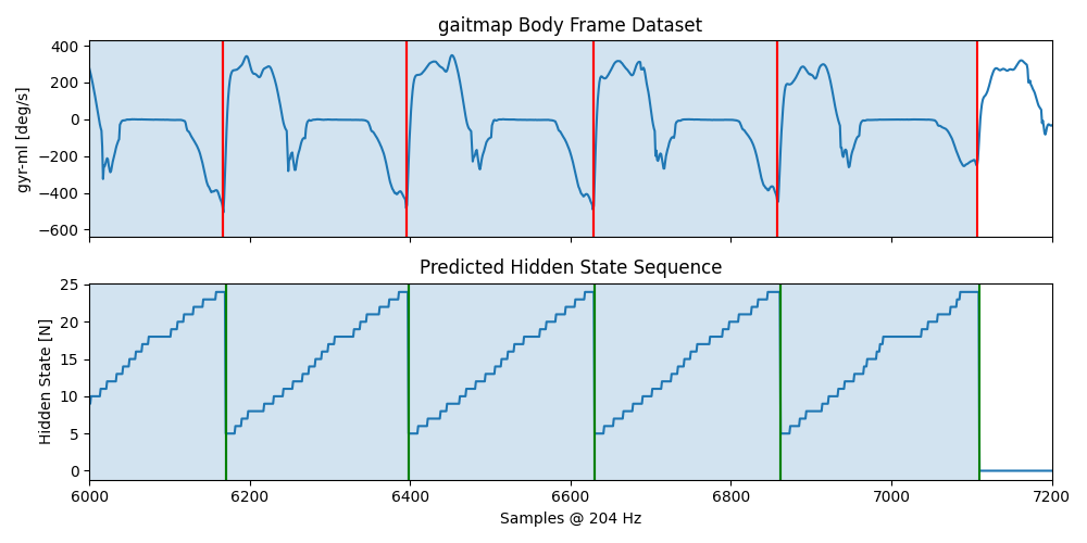
Plotting the Results#
sensor = "left_sensor"

fig, axs = plt.subplots(nrows=2, sharex=True, figsize=(10, 5))
axs[0].set_title("gaitmap Body Frame Dataset")
axs[0].plot(bf_data.reset_index(drop=True)[sensor]["gyr_ml"])
for start, end in hmm.stride_list_["left_sensor"].to_numpy():
    axs[0].axvline(start, c="r")
    axs[0].axvline(end, c="r")
    axs[0].axvspan(start, end, alpha=0.2)
axs[0].set_ylabel("gyr-ml [deg/s]")

axs[1].set_title("Predicted Hidden State Sequence")
axs[1].plot(hmm.hidden_state_sequence_[sensor])
for start, end in hmm.matches_start_end_original_[sensor]:
    axs[1].axvline(start, c="g")
    axs[1].axvline(end, c="g")
    axs[1].axvspan(start, end, alpha=0.2)
axs[1].set_ylabel("Hidden State [N]")

axs[1].set_xlabel("Samples @ %d Hz" % sampling_rate_hz)
plt.xlim([6000, 7200])
fig.tight_layout()
plt.show()
Total running time of the script: ( 0 minutes 6.260 seconds)
Estimated memory usage: 9 MB