Note
Click here to download the full example code
Herzer event detection#
This example illustrates how the gait event detection by the HerzerEventDetection
can be used to detect gait events within a list of strides and the corresponding IMU signal.
The structure of this example will be very similar to the example for the
RamppEventDetection.
Checkout this example for more details.
Getting some example data#
from gaitmap.example_data import get_healthy_example_imu_data

data = get_healthy_example_imu_data()
sampling_rate_hz = 204.8
data.sort_index(axis=1).head(1)
Getting the example stride list#
from gaitmap.example_data import get_healthy_example_stride_borders

stride_list = get_healthy_example_stride_borders()

stride_list["left_sensor"].head()
Preparing the data#
The data is expected to be in the gaitmap BF to be able to use the same rules for the left and the right foot.
from gaitmap.utils.coordinate_conversion import convert_to_fbf

bf_data = convert_to_fbf(data, left_like="left_", right_like="right_")
Applying the event detection#
First we need to initialize the Herzer event detection. In most cases it is sufficient to keep all parameters at default.
from gaitmap.event_detection import HerzerEventDetection

ed = HerzerEventDetection()
# apply the event detection to the data
ed = ed.detect(data=bf_data, stride_list=stride_list, sampling_rate_hz=sampling_rate_hz)
Inspecting the results#
The main output is the min_vel_event_list_, which contains the samples of initial contact (ic), terminal contact
(tc), and minimal velocity (min_vel) formatted in a way that can be directly used for a stride-level trajectory
reconstruction.
The start sample of each stride corresponds to the min_vel sample of that stride and the end sample corresponds to the
min_vel sample of the subsequent stride.
Furthermore, the min_vel_event_list_ list provides the pre_ic which is the ic event of the previous stride in the
stride list.
As we passed a dataset with two sensors, the output will be a dictionary.
min_vel_events_left = ed.min_vel_event_list_["left_sensor"]
print(f"Gait events for {len(min_vel_events_left)} min_vel strides were detected.")
min_vel_events_left.head()
Gait events for 26 min_vel strides were detected.
As a secondary output we get the segmented_event_list_, which holds the same event information than the
min_vel_event_list_, but the start and the end of each stride are unchanged compared to the input.
This also means that no strides are removed due to the conversion step explained below.
segmented_events_left = ed.segmented_event_list_["left_sensor"]
print(f"Gait events for {len(segmented_events_left)} segmented strides were detected.")
segmented_events_left.head()
Gait events for 28 segmented strides were detected.
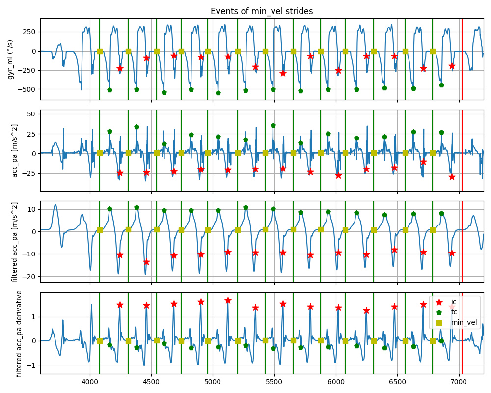
To get a better understanding of the results, we can plot the data and the gait events.
The top row shows the gyr_ml axis, the middle row the acc_pa axis, the third row shows the lowpass filtered
acc_pa axis and the bottom row the lowpass filtered derivative of the acc_pa signal, that is used to find the ic
point.
The vertical lines show the start and end of the strides that are overlapping with the min_vel samples. Only the second sequence of strides of the left foot are shown.
import matplotlib.pyplot as plt
import numpy as np

# calculate the filtered signal:
acc_pa_low = ed.ic_lowpass_filter.filter(
    bf_data.reset_index(drop=True)["left_sensor"]["acc_pa"], sampling_rate_hz=sampling_rate_hz
).filtered_data_
acc_pa_der = np.diff(acc_pa_low)

fig, axs = plt.subplots(4, sharex=True, figsize=(10, 8))
axs_data = [
    bf_data.reset_index(drop=True)["left_sensor"][["gyr_ml"]].to_numpy(),
    bf_data.reset_index(drop=True)["left_sensor"][["acc_pa"]].to_numpy(),
    acc_pa_low,
    acc_pa_der,
]

ic_idx = ed.min_vel_event_list_["left_sensor"]["ic"].to_numpy().astype(int)
tc_idx = ed.min_vel_event_list_["left_sensor"]["tc"].to_numpy().astype(int)
min_vel_idx = ed.min_vel_event_list_["left_sensor"]["min_vel"].to_numpy().astype(int)

for ax, data in zip(axs, axs_data):
    ax.plot(data)
    for _i, stride in ed.min_vel_event_list_["left_sensor"].iterrows():
        ax.axvline(stride["start"], color="g")
        ax.axvline(stride["end"], color="r")

    for (m, s, c, l), pos in zip(
        [("*", 100, "r", "ic"), ("p", 50, "g", "tc"), ("s", 50, "y", "min_vel")], [ic_idx, tc_idx, min_vel_idx]
    ):
        ax.scatter(pos, data[pos], marker=m, s=s, color=c, zorder=3, label=l)

    ax.grid(True)

axs[0].set_title("Events of min_vel strides")
axs[0].set_ylabel("gyr_ml (°/s)")
axs[1].set_ylabel("acc_pa [m/s^2]")
axs[2].set_ylabel("filtered acc_pa [m/s^2]")
axs[3].set_ylabel("filtered acc_pa derivative")
axs[0].set_xlim(3600, 7200)
plt.legend(loc="best")

fig.tight_layout()
fig.show()
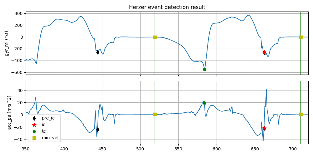
To better understand the concept of ic and pre_ic, let’s take a closer look at the data and zoom in a bit more. We can see now that every stride has a pre_ic and especially in case of the first stride of a sequence this pre_ic is not an ic for any stride. It only serves as a pre_ic for the subsequent stride.
fig, (ax1, ax2) = plt.subplots(2, sharex=True, figsize=(10, 5))
ax1.plot(bf_data.reset_index(drop=True)["left_sensor"][["gyr_ml"]])
ax2.plot(bf_data.reset_index(drop=True)["left_sensor"][["acc_pa"]])

pre_ic_idx = ed.min_vel_event_list_["left_sensor"]["pre_ic"].to_numpy().astype(int)

for ax, sensor in zip([ax1, ax2], ["gyr_ml", "acc_pa"]):
    for _i, stride in ed.min_vel_event_list_["left_sensor"].iterrows():
        ax.axvline(stride["start"], color="g")
        ax.axvline(stride["end"], color="r")

    ax.scatter(
        pre_ic_idx,
        bf_data["left_sensor"][sensor].to_numpy()[pre_ic_idx],
        marker="d",
        s=50,
        color="k",
        zorder=3,
        label="pre_ic",
    )

    ax.scatter(
        ic_idx,
        bf_data["left_sensor"][sensor].to_numpy()[ic_idx],
        marker="*",
        s=100,
        color="r",
        zorder=3,
        label="ic",
    )

    ax.scatter(
        tc_idx,
        bf_data["left_sensor"][sensor].to_numpy()[tc_idx],
        marker="p",
        s=50,
        color="g",
        zorder=3,
        label="tc",
    )

    ax.scatter(
        min_vel_idx,
        bf_data["left_sensor"][sensor].to_numpy()[min_vel_idx],
        marker="s",
        s=50,
        color="y",
        zorder=3,
        label="min_vel",
    )

    ax.grid(True)

ax1.set_title("Herzer event detection result")
ax1.set_ylabel("gyr_ml (°/s)")
ax2.set_ylabel("acc_pa [m/s^2]")
ax1.set_xlim(350, 720)
plt.legend(loc="best")

fig.tight_layout()
fig.show()
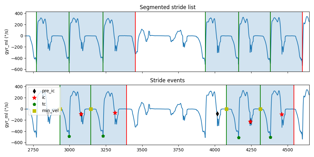
Furthermore, breaks in continuous gait sequences (with continuous subsequent strides according to the stride_list)
are detected and the first (segmented) stride of each sequence is dropped.
This is required due to the shift of stride borders between the stride_list and the min_vel_event_list_.
Thus, the dropped first segmented stride of a continuous sequence only provides a pre_ic and a min_vel sample for
the first stride in the min_vel_event_list_.
Therefore, the min_vel_event_list_ list has one stride less than the segmented_event_list_.
ed2 = HerzerEventDetection()
segmented_stride_list = stride_list["left_sensor"].iloc[[11, 12, 13, 14, 15, 16]]
ed2.detect(
    data=bf_data["left_sensor"],
    sampling_rate_hz=sampling_rate_hz,
    stride_list=segmented_stride_list,
)

fig, (ax1, ax2) = plt.subplots(2, sharex=True, figsize=(10, 5))

sensor_axis = "gyr_ml"

ax1.plot(bf_data.reset_index(drop=True)["left_sensor"][sensor_axis])
for _i, stride in segmented_stride_list.iterrows():
    ax1.axvline(stride["start"], color="g")
    ax1.axvline(stride["end"], color="r")
    ax1.axvspan(stride["start"], stride["end"], alpha=0.2)

ax2.plot(bf_data.reset_index(drop=True)["left_sensor"][sensor_axis])

ic_idx = ed2.min_vel_event_list_["ic"].to_numpy().astype(int)
tc_idx = ed2.min_vel_event_list_["tc"].to_numpy().astype(int)
min_vel_idx = ed2.min_vel_event_list_["min_vel"].to_numpy().astype(int)
pre_ic_idx = ed2.min_vel_event_list_["pre_ic"].to_numpy().astype(int)

for _i, stride in ed2.min_vel_event_list_.iterrows():
    ax2.axvline(stride["start"], color="g")
    ax2.axvline(stride["end"], color="r")
    ax2.axvspan(stride["start"], stride["end"], alpha=0.2)

ax2.scatter(
    pre_ic_idx,
    bf_data["left_sensor"][sensor_axis].to_numpy()[pre_ic_idx],
    marker="d",
    s=50,
    color="k",
    zorder=3,
    label="pre_ic",
)

ax2.scatter(
    ic_idx,
    bf_data["left_sensor"][sensor_axis].to_numpy()[ic_idx],
    marker="*",
    s=100,
    color="r",
    zorder=3,
    label="ic",
)

ax2.scatter(
    tc_idx,
    bf_data["left_sensor"][sensor_axis].to_numpy()[tc_idx],
    marker="p",
    s=50,
    color="g",
    zorder=3,
    label="tc",
)

ax2.scatter(
    min_vel_idx,
    bf_data["left_sensor"][sensor_axis].to_numpy()[min_vel_idx],
    marker="s",
    s=50,
    color="y",
    zorder=3,
    label="min_vel",
)

ax1.set_title("Segmented stride list")
ax1.set_ylabel("gyr_ml (°/s)")
ax2.set_title("Stride events")
ax2.set_ylabel("gyr_ml (°/s)")
ax1.set_xlim(2700, 4650)
fig.tight_layout()

plt.legend(loc="upper left")
fig.show()
Total running time of the script: ( 0 minutes 3.416 seconds)
Estimated memory usage: 9 MB