Constrained BarthDtw stride segmentation

This example illustrates how subsequent DTW with local warping constraints can be more effective than simple DTW for stride segmentation in a continuous DTW signal.

In a traditional dtw approach (as used by [1] and implemented by BarthDtw) it is possible to match extremely short or extremely long signals by stretching the data or the template, respectively. These matches are usually False-positives. In BarthDtw we can use postproccessing steps to remove these matches. However, because this selection occurs after the actual DTW, it is not possible to recover matches that were prevented by the existence of such false matches in the first place.

A very typical error that occurs (see below) is that the warping path only covers part of the stride. This is typically either the part from the TC to IC (the start is correct, end not) or from IC to TC (the end is correct, start not). In both cases, basically half of the template is warped onto a very small number of actual signal samples. This is often caused by slight abnormalities in either the first or the second half of the stride, which makes it unfeasible to include them in the stride.

In normal (aka not subsequence) DTW such “short-cuts” can be prevented by adding a mask to the distance matrix, that constrains the possible regions the warping path can go through. However, this is only possible, if the start and the endpoint of the path is known beforehand. Therefore, these “global” constrains can not be used in subsequence-DTW. But, it is possible to use local constraints, that prohibit that a single sample of the template is mapped to >N samples of the signal or that a single sample of the signal is mapped to >M samples of the template.

These constraints are used by ConstrainedBarthDtw via the parameters max_template_stretch_ms and max_signal_stretch_ms. Note that these parameters can also be used in BarthDtw, but the ConstrainedBarthDtw has already sensible defaults set.

[1]

Barth, J., Oberndorfer, C., Kugler, P., Schuldhaus, D., Winkler, J., Klucken, J., & Eskofier, B. (2013). Subsequence dynamic time warping as a method for robust step segmentation using gyroscope signals of daily life activities. Proceedings of the Annual International Conference of the IEEE Engineering in Medicine and Biology Society, EMBS, 6744–6747. https://doi.org/10.1109/EMBC.2013.6611104

import matplotlib.pyplot as plt
import numpy

numpy.random.seed(0)

Getting some example data

For this we load a special dataset, where the error described above was extremely noticeable. While it is hard to pinpoint, why exactly this is the case, it appears to be due to the deep dip of the gyr_ml signal around the IC.

from gaitmap.example_data import get_ms_example_imu_data
from gaitmap.utils.coordinate_conversion import convert_to_fbf

data = get_ms_example_imu_data()
sampling_rate_hz = 102.4
bf_data = convert_to_fbf(data, left_like="left_", right_like="right_")

Establish a baseline

Before testing the local constraints, we use the simple BarthDtw to visualise the issue. We will remove the min_match_length_s post-processing step, so that we can see the warping-paths of the mismatches. Note, that we only use the “gyr_ml” and “gyr_si” axis for matching. In this (and many other cases), this can help recognise more strides correctly, with the risk of segmenting “non-strides” as well.

from gaitmap.stride_segmentation import BarthDtw, BarthOriginalTemplate, ConstrainedBarthDtw

dtw = BarthDtw(BarthOriginalTemplate(use_cols=("gyr_ml", "gyr_si")), min_match_length_s=None)
# Apply the dtw to the data
dtw = dtw.segment(data=bf_data, sampling_rate_hz=sampling_rate_hz)

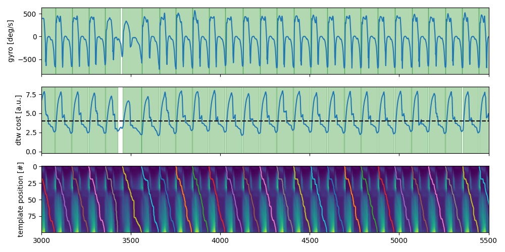
Visualize the baseline

def plot_dtw(dtw, sensor="left_sensor") -> None:
    fig, axs = plt.subplots(nrows=3, sharex=True, figsize=(10, 5))
    dtw.data[sensor]["gyr_ml"].reset_index(drop=True).plot(ax=axs[0])
    axs[0].set_ylabel("gyro [deg/s]")
    axs[1].plot(dtw.cost_function_[sensor])
    axs[1].set_ylabel("dtw cost [a.u.]")
    axs[1].axhline(dtw.max_cost, color="k", linestyle="--")
    axs[2].imshow(dtw.acc_cost_mat_[sensor], aspect="auto")
    axs[2].set_ylabel("template position [#]")
    for p in dtw.paths_[sensor]:
        axs[2].plot(p.T[1], p.T[0])
    for s in dtw.matches_start_end_original_[sensor]:
        axs[1].axvspan(*s, alpha=0.3, color="g")
    for _, s in dtw.stride_list_[sensor][["start", "end"]].iterrows():
        axs[0].axvspan(*s, alpha=0.3, color="g")

    axs[0].set_xlim(3000, 5500)
    axs[0].set_xlabel("time [#]")
    fig.tight_layout()
    fig.show()


plot_dtw(dtw)

Constrained DTW

As it can be seen above, we have a lot of TC-IC mismatches. They result in a steep vertical part of the warping path. We can mitigate that behaviour by restricting the number of template samples that can be warped to the same signal sample.

This can be controlled by the max_template_stretch_ms parameter. It expects a value in “ms” to be independent of the sampling rate. This means if we only want to allow 10 matches (but not 11 or more) with the same signal sample, we need to set the constrain to 11 / sampling_rate_hz / 1000, which means approx 110 ms at a sampling rate of 102.4 Hz.

As seen below, this fixes a couple of the mismatches. We can see the effect very clearly in the cost function, too. Before there were two minima per stride, indicating that the TC-IC match had a very similar cost to the full match. Now only the actual end of the stride has a feasible cost. However, in the strides that are still not detected, the optimal warping path ends at the correct position, by starts in the middle of the stride at the IC (i.e. a IC-TC mismatch).

cdtw = BarthDtw(
    BarthOriginalTemplate(use_cols=("gyr_ml", "gyr_si")),
    max_template_stretch_ms=110,
    max_signal_stretch_ms=None,
    min_match_length_s=None,
)
cdtw = cdtw.segment(data=bf_data, sampling_rate_hz=sampling_rate_hz)

plot_dtw(cdtw)

The Constrained DTW class

To make it easy to constrained dtw with sensible defaults, the ConstrainedBarthDtw class exists. It uses 120 ms for both the signal and the template stretch. Note that you still need to change the template columns to reproduce the results from above.

default_cdtw = ConstrainedBarthDtw(
    BarthOriginalTemplate(use_cols=("gyr_ml", "gyr_si")),
    min_match_length_s=None,
    max_signal_stretch_ms=None,
)
default_cdtw = default_cdtw.segment(data=bf_data, sampling_rate_hz=sampling_rate_hz)

plot_dtw(default_cdtw)

Estimated memory usage: 49 MB