BarthDtw stride segmentation

This example illustrates how subsequent DTW implemented by the BarthDtw can be used to detect strides in a continuous signal of an IMU signal. The used implementation is based on the work of Barth et al [1] and adds a set of postprocessing methods that aim to reduce the chance of false positives.

[1]

Barth, J., Oberndorfer, C., Kugler, P., Schuldhaus, D., Winkler, J., Klucken, J., & Eskofier, B. (2013). Subsequence dynamic time warping as a method for robust step segmentation using gyroscope signals of daily life activities. Proceedings of the Annual International Conference of the IEEE Engineering in Medicine and Biology Society, EMBS, 6744–6747. https://doi.org/10.1109/EMBC.2013.6611104

import matplotlib.pyplot as plt
import numpy

numpy.random.seed(0)

Getting some example data

For this we take some example data that contains the regular walking movement during a 2x20m walk test of a healthy subject. The IMU signals are already rotated so that they align with the gaitmap SF coordinate system. The data contains information from two sensors - one from the right and one from the left foot.

from gaitmap.example_data import get_healthy_example_imu_data

data = get_healthy_example_imu_data()
sampling_rate_hz = 204.8
data.sort_index(axis=1).head(1)

sensor	left_sensor						right_sensor
axis	acc_x	acc_y	acc_z	gyr_x	gyr_y	gyr_z	acc_x	acc_y	acc_z	gyr_x	gyr_y	gyr_z
0.0	0.880811	2.762208	9.40865	-0.112402	-0.032157	-0.062261	0.311553	-2.398646	9.513275	-0.323037	0.084604	-0.025288

Selecting a template

This library ships with the template that was originally used by Barth et al. It is generated based on manually segmented strides from healthy participants and PD patients. This template is used by default by BarthDtw, but we will load it manually in this example.

from gaitmap.stride_segmentation import BarthOriginalTemplate

template = BarthOriginalTemplate()
template.get_data().plot()
plt.xlabel("Time [#]")
plt.ylabel("gyro [deg/s]")
plt.show()

Preparing the data

The template only makes use of the gyro information. Further, if you use this template in the DTW, your data is expected to be in the gaitmap BF to be able to use the same template for the left and the right foot. Therefore, we need to transform the dataset into the body frame.

from gaitmap.utils.coordinate_conversion import convert_to_fbf

# We use the `..._like` parameters to identify the data of the left and the right foot based on the name of the sensor.
bf_data = convert_to_fbf(data, left_like="left_", right_like="right_")

Applying the DTW

First we need to initialize the DTW. In most cases it is sufficient to keep all parameters at default. However, if you experience any issues you should start modifying the parameters, starting by max_cost, as it has the highest influence on the result.

from gaitmap.stride_segmentation import BarthDtw

dtw = BarthDtw(template=template)
# Apply the dtw to the data
dtw = dtw.segment(data=bf_data, sampling_rate_hz=sampling_rate_hz)

Inspecting the results

The main output is the stride_list_, which contains the start and the end of all identified strides. As we passed a dataset with two sensors, the output will be a dictionary.

stride_list_left = dtw.stride_list_["left_sensor"]
print(f"{len(stride_list_left)} strides were detected.")
stride_list_left.head()

28 strides were detected.

	start	end
s_id
0	364	584
1	584	802
2	802	1023
3	1023	1242
4	1242	1458

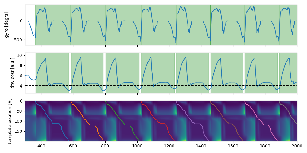
To get a better understanding of the results, we can plot additional information about the results. The top row shows the gyr_ml axis with the segmented strides plotted on top. They are postprocessed to snap to the closed data minimum. In the second row the cost function of the DTW is plotted. Each minimum marks a potential end of a stride. The black dotted line indicates the used max_cost threshold to search for stride candidates. The drawn boxes show the raw result of the DTW without the snap-to-min postprocessing. The third row shows the entire accumulated cost matrix and the path each stride takes through the cost matrix to achieve minimal cost.

Only the first couple of strides of the left foot are shown.

sensor = "left_sensor"
fig, axs = plt.subplots(nrows=3, sharex=True, figsize=(10, 5))
dtw.data[sensor]["gyr_ml"].reset_index(drop=True).plot(ax=axs[0])
axs[0].set_ylabel("gyro [deg/s]")
axs[1].plot(dtw.cost_function_[sensor])
axs[1].set_ylabel("dtw cost [a.u.]")
axs[1].axhline(dtw.max_cost, color="k", linestyle="--")
axs[2].imshow(dtw.acc_cost_mat_[sensor], aspect="auto")
axs[2].set_ylabel("template position [#]")
for p in dtw.paths_[sensor]:
    axs[2].plot(p.T[1], p.T[0])
for s in dtw.matches_start_end_original_[sensor]:
    axs[1].axvspan(*s, alpha=0.3, color="g")
for _, s in dtw.stride_list_[sensor][["start", "end"]].iterrows():
    axs[0].axvspan(*s, alpha=0.3, color="g")

axs[0].set_xlim(300, 2000)
axs[0].set_xlabel("time [#]")
fig.tight_layout()
fig.show()

Estimated memory usage: 39 MB