Note
Click here to download the full example code
ZUPT Dependency of the Trajectory Estimation#
The estimation of the trajectory using the Kalman filter is heavily dependend on the ZUPT detection [1]. For this reason we provide various ZUPT detection methods in gaitmap. Each of these methods has further parameters, that can (and should) be tuned to the specific data.
In this example we show, how to Gridsearch the Parameter space of the ZUPT detection methods to find the best
combination.
This makes heavy use of the tpcp optimization methods and the Gridsearch used here can be substituted by any other
optimize method.
This is also a great example of how to use the tpcp optimization methods in combination with gaitmap.
import pandas as pd
The Data#
We gonna use the healthy example IMU data to find the best settings.
To use this data with tpcp, we need to wrap it into a Dataset class.
For more details about this see the gridsearch or the custom dataset
example.
Here we will just copy and paste the dataset used in the gridsearch example and add an additional mocap_trajectory_
property that allows access to the respective mocap reference data.
from tpcp import Dataset

from gaitmap.example_data import get_healthy_example_imu_data, get_healthy_example_mocap_data
The Dataset#
To use any tpcp features, we need to wrap our data into a dataset object.
For this we need an index.
Usually you create this by iterating a directory of datafiles you have and list out all participants/tests.
To keep things simple we just use data from one participant and one test, but treat the left and right foot
as two independent datasets.
This is something you would not normally do.
class HealthyImu(Dataset):
    @property
    def sampling_rate_hz(self) -> float:
        return 204.8

    @property
    def data(self) -> pd.DataFrame:
        self.assert_is_single(None, "data")
        return get_healthy_example_imu_data()[self.index.iloc[0]["foot"] + "_sensor"]

    @property
    def mocap_trajectory_(self) -> pd.DataFrame:
        self.assert_is_single(None, "data")
        df = get_healthy_example_mocap_data().filter(like=self.group_label.foot[0].upper())
        # This strips the L_/R_ prefix
        df.columns = pd.MultiIndex.from_tuples((m[2:], a) for m, a in df.columns)
        return df

    def create_index(self) -> pd.DataFrame:
        return pd.DataFrame({"foot": ["left", "right"]})
Setting up a pipeline#
We start by setting up a pipeline, that we can use to estimate the trajectory.
It takes the Zupt method as parameter and internally uses RtsKalman to estimate the trajectory.
from tpcp import Pipeline, cf
from typing_extensions import Self

from gaitmap.base import BaseZuptDetector
from gaitmap.trajectory_reconstruction import RtsKalman
from gaitmap.zupt_detection import ShoeZuptDetector


class TrajectoryPipeline(Pipeline[HealthyImu]):
    trajectory_: pd.DataFrame

    def __init__(self, zupt_method: BaseZuptDetector = cf(ShoeZuptDetector())) -> None:
        self.zupt_method = zupt_method

    def run(self, datapoint: HealthyImu) -> Self:
        rts_kalman = RtsKalman(zupt_detector=self.zupt_method)
        self.trajectory_ = rts_kalman.estimate(datapoint.data, sampling_rate_hz=datapoint.sampling_rate_hz).position_
        return self
Scorer#
To decide what parameters we consider good, we need a score function. In this case (to keep things simple), we are going to take the walking distance estimated by the kalman filter. In the example data, the participant walked 20 m in one direction, turned around and walked back. Hence, we are going to check how close our results are to the 20 m. To be more precise, we are going to calculate the actual walking distance from the associated mocap data.
import numpy as np


def score(pipeline: TrajectoryPipeline, datapoint: HealthyImu) -> float:
    pipeline.safe_run(datapoint)
    trajectory = pipeline.trajectory_[["pos_x", "pos_y"]]
    walk_distance = np.max(np.linalg.norm(trajectory, axis=1))
    ground_truth_traj = datapoint.mocap_trajectory_["TOE"][["x", "y"]]
    ground_truth_walk_distance = np.max(np.linalg.norm(ground_truth_traj - ground_truth_traj.iloc[0], axis=1))
    return np.abs(walk_distance - ground_truth_walk_distance / 1000)


from sklearn.model_selection import ParameterGrid
Gridsearch#
Now we can set up a simple GridSearch.
We just need to specify the parameters we want to use.
Note, we use the __ syntax to set parameters of the nested zupt_method object
from tpcp.optimize import GridSearch

# Para-grid used to optimize the default values of the ShoeZuptDetector
# paras = ParameterGrid(
#     {
#         "zupt_method__inactive_signal_threshold": np.logspace(3, 10, 100),
#         "zupt_method__acc_noise_variance": np.logspace(-10, -3, 10),
#         "zupt_method__gyr_noise_variance": np.logspace(-10, -3, 10),
#     }
# )

# Shorter para grid for the example
paras = ParameterGrid(
    {
        "zupt_method__inactive_signal_threshold": np.logspace(5, 10, 10),
    }
)
Then we can simply run the GridSearch.
Note, that we specify -score for return_optimized, as we want to select the smallest error as best.
gs = GridSearch(TrajectoryPipeline(), paras, scoring=score, return_optimized="-score")
gs.optimize(HealthyImu())
Parameter Combinations:   0%|          | 0/10 [00:00<?, ?it/s]

Datapoints:   0%|          | 0/2 [00:00<?, ?it/s]

Datapoints:  50%|#####     | 1/2 [00:00<00:00,  6.77it/s]

Datapoints: 100%|##########| 2/2 [00:00<00:00,  7.70it/s]
Datapoints: 100%|##########| 2/2 [00:00<00:00,  7.53it/s]

Parameter Combinations:  10%|#         | 1/10 [00:00<00:02,  3.61it/s]

Datapoints:   0%|          | 0/2 [00:00<?, ?it/s]

Datapoints:  50%|#####     | 1/2 [00:00<00:00,  8.54it/s]

Datapoints: 100%|##########| 2/2 [00:00<00:00,  8.57it/s]
Datapoints: 100%|##########| 2/2 [00:00<00:00,  8.55it/s]

Parameter Combinations:  20%|##        | 2/10 [00:00<00:02,  3.91it/s]

Datapoints:   0%|          | 0/2 [00:00<?, ?it/s]

Datapoints:  50%|#####     | 1/2 [00:00<00:00,  8.60it/s]

Datapoints: 100%|##########| 2/2 [00:00<00:00,  8.61it/s]
Datapoints: 100%|##########| 2/2 [00:00<00:00,  8.60it/s]

Parameter Combinations:  30%|###       | 3/10 [00:00<00:01,  4.03it/s]

Datapoints:   0%|          | 0/2 [00:00<?, ?it/s]

Datapoints:  50%|#####     | 1/2 [00:00<00:00,  8.58it/s]

Datapoints: 100%|##########| 2/2 [00:00<00:00,  8.61it/s]
Datapoints: 100%|##########| 2/2 [00:00<00:00,  8.59it/s]

Parameter Combinations:  40%|####      | 4/10 [00:00<00:01,  4.08it/s]

Datapoints:   0%|          | 0/2 [00:00<?, ?it/s]

Datapoints:  50%|#####     | 1/2 [00:00<00:00,  8.62it/s]

Datapoints: 100%|##########| 2/2 [00:00<00:00,  8.63it/s]
Datapoints: 100%|##########| 2/2 [00:00<00:00,  8.62it/s]

Parameter Combinations:  50%|#####     | 5/10 [00:01<00:01,  4.12it/s]

Datapoints:   0%|          | 0/2 [00:00<?, ?it/s]

Datapoints:  50%|#####     | 1/2 [00:00<00:00,  8.68it/s]

Datapoints: 100%|##########| 2/2 [00:00<00:00,  8.39it/s]
Datapoints: 100%|##########| 2/2 [00:00<00:00,  8.42it/s]

Parameter Combinations:  60%|######    | 6/10 [00:01<00:00,  4.11it/s]

Datapoints:   0%|          | 0/2 [00:00<?, ?it/s]

Datapoints:  50%|#####     | 1/2 [00:00<00:00,  8.07it/s]

Datapoints: 100%|##########| 2/2 [00:00<00:00,  7.97it/s]
Datapoints: 100%|##########| 2/2 [00:00<00:00,  7.98it/s]

Parameter Combinations:  70%|#######   | 7/10 [00:01<00:00,  4.03it/s]

Datapoints:   0%|          | 0/2 [00:00<?, ?it/s]

Datapoints:  50%|#####     | 1/2 [00:00<00:00,  7.44it/s]

Datapoints: 100%|##########| 2/2 [00:00<00:00,  7.53it/s]
Datapoints: 100%|##########| 2/2 [00:00<00:00,  7.51it/s]

Parameter Combinations:  80%|########  | 8/10 [00:02<00:00,  3.90it/s]

Datapoints:   0%|          | 0/2 [00:00<?, ?it/s]

Datapoints:  50%|#####     | 1/2 [00:00<00:00,  7.08it/s]

Datapoints: 100%|##########| 2/2 [00:00<00:00,  7.01it/s]
Datapoints: 100%|##########| 2/2 [00:00<00:00,  7.01it/s]

Parameter Combinations:  90%|######### | 9/10 [00:02<00:00,  3.74it/s]

Datapoints:   0%|          | 0/2 [00:00<?, ?it/s]

Datapoints:  50%|#####     | 1/2 [00:00<00:00,  6.78it/s]

Datapoints: 100%|##########| 2/2 [00:00<00:00,  6.82it/s]
Datapoints: 100%|##########| 2/2 [00:00<00:00,  6.81it/s]

Parameter Combinations: 100%|##########| 10/10 [00:02<00:00,  3.60it/s]
Parameter Combinations: 100%|##########| 10/10 [00:02<00:00,  3.84it/s]

GridSearch(n_jobs=None, parameter_grid=<sklearn.model_selection._search.ParameterGrid object at 0x7efee12f9a90>, pipeline=TrajectoryPipeline(zupt_method=ShoeZuptDetector(acc_noise_variance=3.5e-09, gyr_noise_variance=1.3e-07, inactive_signal_threshold=2310129700, window_length_s=0.15, window_overlap=0.5, window_overlap_samples=None)), pre_dispatch='n_jobs', progress_bar=True, return_optimized='-score', scoring=<function score at 0x7efee3638af0>)
Results#
{'score': array([1955.731, 1955.731, 1955.731, 1955.731, 1955.731, 1115.828,    3.353,    0.413,    0.102,    0.144]), 'rank_score': array([ 1,  1,  1,  1,  1,  6,  7,  8, 10,  9], dtype=int32), 'single_score': [[2128.724719930634, 1782.7378860920396], [2128.724719930634, 1782.7378860920396], [2128.724719930634, 1782.7378860920396], [2128.724719930634, 1782.7378860920396], [2128.724719930634, 1782.7378860920396], [2128.724719930634, 102.93052426695826], [4.072482285010359, 2.634029915951018], [0.8049839003173851, 0.021696130797351998], [0.1275696898520522, 0.07585134112428094], [0.2776723925921978, 0.00983052935283979]], 'data_labels': [[HealthyImuGroupLabel(foot='left'), HealthyImuGroupLabel(foot='right')], [HealthyImuGroupLabel(foot='left'), HealthyImuGroupLabel(foot='right')], [HealthyImuGroupLabel(foot='left'), HealthyImuGroupLabel(foot='right')], [HealthyImuGroupLabel(foot='left'), HealthyImuGroupLabel(foot='right')], [HealthyImuGroupLabel(foot='left'), HealthyImuGroupLabel(foot='right')], [HealthyImuGroupLabel(foot='left'), HealthyImuGroupLabel(foot='right')], [HealthyImuGroupLabel(foot='left'), HealthyImuGroupLabel(foot='right')], [HealthyImuGroupLabel(foot='left'), HealthyImuGroupLabel(foot='right')], [HealthyImuGroupLabel(foot='left'), HealthyImuGroupLabel(foot='right')], [HealthyImuGroupLabel(foot='left'), HealthyImuGroupLabel(foot='right')]], 'score_time': array([0.275, 0.24 , 0.238, 0.238, 0.238, 0.243, 0.256, 0.272, 0.291, 0.299]), 'param_zupt_method__inactive_signal_threshold': masked_array(data=[100000.0, 359381.36638046254, 1291549.6650148826, 4641588.833612782, 16681005.372000592, 59948425.03189409, 215443469.00318864, 774263682.6811278,
                   2782559402.2071257, 10000000000.0],
             mask=[False, False, False, False, False, False, False, False, False, False],
       fill_value='?',
            dtype=object), 'params': [{'zupt_method__inactive_signal_threshold': 100000.0}, {'zupt_method__inactive_signal_threshold': 359381.36638046254}, {'zupt_method__inactive_signal_threshold': 1291549.6650148826}, {'zupt_method__inactive_signal_threshold': 4641588.833612782}, {'zupt_method__inactive_signal_threshold': 16681005.372000592}, {'zupt_method__inactive_signal_threshold': 59948425.03189409}, {'zupt_method__inactive_signal_threshold': 215443469.00318864}, {'zupt_method__inactive_signal_threshold': 774263682.6811278}, {'zupt_method__inactive_signal_threshold': 2782559402.2071257}, {'zupt_method__inactive_signal_threshold': 10000000000.0}]}
We can also specifically get the best results
print(pd.DataFrame(results))
print(gs.best_params_)
print(gs.best_score_)
         score  ...                                             params
0  1955.731303  ...  {'zupt_method__inactive_signal_threshold': 100...
1  1955.731303  ...  {'zupt_method__inactive_signal_threshold': 359...
2  1955.731303  ...  {'zupt_method__inactive_signal_threshold': 129...
3  1955.731303  ...  {'zupt_method__inactive_signal_threshold': 464...
4  1955.731303  ...  {'zupt_method__inactive_signal_threshold': 166...
5  1115.827622  ...  {'zupt_method__inactive_signal_threshold': 599...
6     3.353256  ...  {'zupt_method__inactive_signal_threshold': 215...
7     0.413340  ...  {'zupt_method__inactive_signal_threshold': 774...
8     0.101711  ...  {'zupt_method__inactive_signal_threshold': 278...
9     0.143751  ...  {'zupt_method__inactive_signal_threshold': 100...

[10 rows x 7 columns]
{'zupt_method__inactive_signal_threshold': 2782559402.2071257}
0.10171051548816656
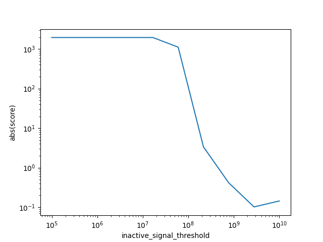
And plot them
import matplotlib.pyplot as plt

result_df = pd.DataFrame(results)
plt.plot(result_df["param_zupt_method__inactive_signal_threshold"], result_df["score"].abs())
plt.xlabel("inactive_signal_threshold")
plt.ylabel("abs(score)")
plt.yscale("log")
plt.xscale("log")
plt.show()
Total running time of the script: ( 0 minutes 4.467 seconds)
Estimated memory usage: 9 MB